Adjusting radar-base rainfall estimates by rain gauge observations#
Background#
There are various ways to correct specific errors and artifacts in radar-based quantitative precipitation estimates (radar QPE). Alternatively, you might want to correct your radar QPE regardless of the error source - by using ground truth, or, more specifically, rain gauge observations. Basically, you define the error of your radar QPE at a rain gauge location by the discrepancy between rain gauge observation (considered as “the truth”) and radar QPE at that very location. Whether you consider this “discrepancy” as an additive or multiplicative error is somehow arbitrary - typically, it’s a mix of both. If you quantify this error at various locations (i.e. rain gauges), you can go ahead and construct correction fields for your radar QPE. You might compute a single correction factor for your entire radar domain (which would e.g. make sense in case of hardware miscalibration), or you might want to compute a spatially variable correction field. This typically implies to interpolate the error in space.
\(\omega radlib\) provides different error models and different spatial interpolation methods to address the adjustment problem. For details, please refer to \(\omega radlib's\) library reference.
[1]:
import wradlib as wrl
import numpy as np
import matplotlib.pyplot as plt

try:
    get_ipython().run_line_magic("matplotlib inline")
except:
    plt.ion()
Example for the 1-dimensional case#
Looking at the 1-D (instead of 2-D) case is more illustrative.
Create synthetic data#
First, we create synthetic data: - true rainfall, - point observations of the truth, - radar observations of the truth.
The latter is disturbed by some kind of error, e.g. a combination between systemtic and random error.
[2]:
# gage and radar coordinates
obs_coords = np.array([5, 10, 15, 20, 30, 45, 65, 70, 77, 90])
radar_coords = np.arange(0, 101)

# true rainfall
np.random.seed(1319622840)
truth = np.abs(1.5 + np.sin(0.075 * radar_coords)) + np.random.uniform(
    -0.1, 0.1, len(radar_coords)
)

# radar error
erroradd = 0.7 * np.sin(0.2 * radar_coords + 10.0)
errormult = 0.75 + 0.015 * radar_coords
noise = np.random.uniform(-0.05, 0.05, len(radar_coords))

# radar observation
radar = errormult * truth + erroradd + noise

# gage observations are assumed to be perfect
obs = truth[obs_coords]

# add a missing value to observations (just for testing)
obs[1] = np.nan
Apply different adjustment methods#
additive error, spatially variable (
AdjustAdd)multiplicative error, spatially variable (
AdjustMultiply)mixed error, spatially variable (
AdjustMixed)multiplicative error, spatially uniform (
AdjustMFB)
[3]:
# number of neighbours to be used
nnear_raws = 3

# adjust the radar observation by additive model
add_adjuster = wrl.adjust.AdjustAdd(obs_coords, radar_coords, nnear_raws=nnear_raws)
add_adjusted = add_adjuster(obs, radar)

# adjust the radar observation by multiplicative model
mult_adjuster = wrl.adjust.AdjustMultiply(
    obs_coords, radar_coords, nnear_raws=nnear_raws
)
mult_adjusted = mult_adjuster(obs, radar)

# adjust the radar observation by AdjustMixed
mixed_adjuster = wrl.adjust.AdjustMixed(obs_coords, radar_coords, nnear_raws=nnear_raws)
mixed_adjusted = mixed_adjuster(obs, radar)

# adjust the radar observation by MFB
mfb_adjuster = wrl.adjust.AdjustMFB(
    obs_coords, radar_coords, nnear_raws=nnear_raws, mfb_args=dict(method="median")
)
mfb_adjusted = mfb_adjuster(obs, radar)
/home/runner/micromamba/envs/wradlib-tests/lib/python3.11/site-packages/wradlib/ipol.py:397: RuntimeWarning: divide by zero encountered in divide
  weights = 1.0 / self.dists**self.p
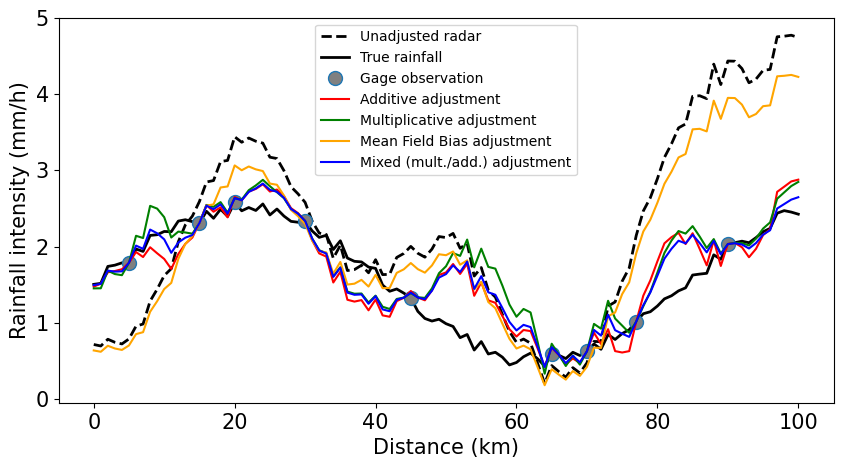
Plot adjustment results#
[4]:
# Enlarge all label fonts
font = {"size": 15}
plt.rc("font", **font)

plt.figure(figsize=(10, 5))
plt.plot(
    radar_coords,
    radar,
    "k",
    linewidth=2.0,
    linestyle="dashed",
    label="Unadjusted radar",
)
plt.plot(
    radar_coords,
    truth,
    "k-",
    linewidth=2.0,
    label="True rainfall",
)
plt.plot(
    obs_coords,
    obs,
    "o",
    markersize=10.0,
    markerfacecolor="grey",
    label="Gage observation",
)
plt.plot(radar_coords, add_adjusted, "-", color="red", label="Additive adjustment")
plt.plot(
    radar_coords, mult_adjusted, "-", color="green", label="Multiplicative adjustment"
)
plt.plot(
    radar_coords, mfb_adjusted, "-", color="orange", label="Mean Field Bias adjustment"
)
plt.plot(
    radar_coords,
    mixed_adjusted,
    "-",
    color="blue",
    label="Mixed (mult./add.) adjustment",
)
plt.xlabel("Distance (km)")
plt.ylabel("Rainfall intensity (mm/h)")
leg = plt.legend(prop={"size": 10})
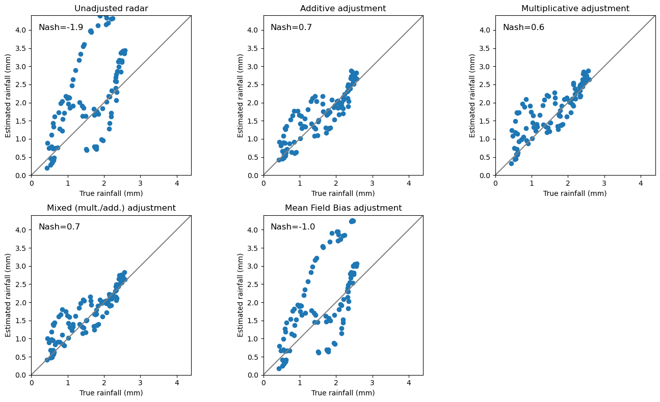
Verification#
We use the verify module to compare the errors of different adjustment approaches.
Here, we compare the adjustment to the “truth”. In practice, we would carry out a cross validation.
[5]:
# Verification for this example
rawerror = wrl.verify.ErrorMetrics(truth, radar)
mfberror = wrl.verify.ErrorMetrics(truth, mfb_adjusted)
adderror = wrl.verify.ErrorMetrics(truth, add_adjusted)
multerror = wrl.verify.ErrorMetrics(truth, mult_adjusted)
mixerror = wrl.verify.ErrorMetrics(truth, mixed_adjusted)
[6]:
# Helper function for scatter plot
def scatterplot(x, y, title=""):
    """Quick and dirty helper function to produce scatter plots"""
    plt.scatter(x, y)
    plt.plot([0, 1.2 * maxval], [0, 1.2 * maxval], "-", color="grey")
    plt.xlabel("True rainfall (mm)")
    plt.ylabel("Estimated rainfall (mm)")
    plt.xlim(0, maxval + 0.1 * maxval)
    plt.ylim(0, maxval + 0.1 * maxval)
    plt.title(title)
[7]:
# Verification reports
maxval = 4.0
# Enlarge all label fonts
font = {"size": 10}
plt.rc("font", **font)
fig = plt.figure(figsize=(14, 8))
ax = fig.add_subplot(231, aspect=1.0)
scatterplot(rawerror.obs, rawerror.est, title="Unadjusted radar")
ax.text(0.2, maxval, "Nash=%.1f" % rawerror.nash(), fontsize=12)
ax = fig.add_subplot(232, aspect=1.0)
scatterplot(adderror.obs, adderror.est, title="Additive adjustment")
ax.text(0.2, maxval, "Nash=%.1f" % adderror.nash(), fontsize=12)
ax = fig.add_subplot(233, aspect=1.0)
scatterplot(multerror.obs, multerror.est, title="Multiplicative adjustment")
ax.text(0.2, maxval, "Nash=%.1f" % multerror.nash(), fontsize=12)
ax = fig.add_subplot(234, aspect=1.0)
scatterplot(mixerror.obs, mixerror.est, title="Mixed (mult./add.) adjustment")
ax.text(0.2, maxval, "Nash=%.1f" % mixerror.nash(), fontsize=12)
ax = fig.add_subplot(235, aspect=1.0)
scatterplot(mfberror.obs, mfberror.est, title="Mean Field Bias adjustment")
ax.text(0.2, maxval, "Nash=%.1f" % mfberror.nash(), fontsize=12)
plt.tight_layout()
Example for the 2-dimensional case#
For the 2-D case, we follow the same approach as before:
create synthetic data: truth, rain gauge observations, radar-based rainfall estimates
apply adjustment methods
verification
The way these synthetic data are created is totally arbitrary - it’s just to show how the methods are applied.
Create 2-D synthetic data#
[8]:
# grid axes
xgrid = np.arange(0, 10)
ygrid = np.arange(20, 30)

# number of observations
num_obs = 10

# create grid
gridshape = len(xgrid), len(ygrid)
grid_coords = wrl.util.gridaspoints(ygrid, xgrid)

# Synthetic true rainfall
truth = np.abs(10.0 * np.sin(0.1 * grid_coords).sum(axis=1))

# Creating radar data by perturbing truth with multiplicative and
# additive error
# YOU CAN EXPERIMENT WITH THE ERROR STRUCTURE
np.random.seed(1319622840)
radar = 0.6 * truth + 1.0 * np.random.uniform(low=-1.0, high=1, size=len(truth))
radar[radar < 0.0] = 0.0

# indices for creating obs from raw (random placement of gauges)
obs_ix = np.random.uniform(low=0, high=len(grid_coords), size=num_obs).astype("i4")

# creating obs_coordinates
obs_coords = grid_coords[obs_ix]

# creating gauge observations from truth
obs = truth[obs_ix]
Apply different adjustment methods#
[9]:
# Mean Field Bias Adjustment
mfbadjuster = wrl.adjust.AdjustMFB(obs_coords, grid_coords)
mfbadjusted = mfbadjuster(obs, radar)

# Additive Error Model
addadjuster = wrl.adjust.AdjustAdd(obs_coords, grid_coords)
addadjusted = addadjuster(obs, radar)

# Multiplicative Error Model
multadjuster = wrl.adjust.AdjustMultiply(obs_coords, grid_coords)
multadjusted = multadjuster(obs, radar)
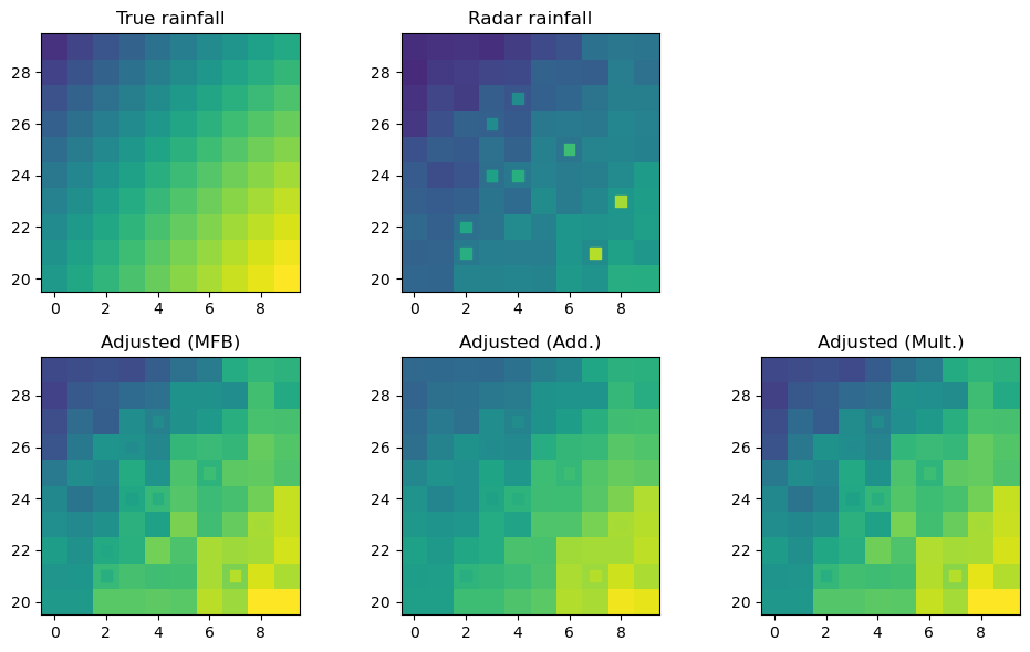
Plot 2-D adjustment results#
[10]:
# Helper functions for grid plots
def gridplot(data, title):
    """Quick and dirty helper function to produce a grid plot"""
    xplot = np.append(xgrid, xgrid[-1] + 1.0) - 0.5
    yplot = np.append(ygrid, ygrid[-1] + 1.0) - 0.5
    grd = ax.pcolormesh(xplot, yplot, data.reshape(gridshape), vmin=0, vmax=maxval)
    ax.scatter(
        obs_coords[:, 0],
        obs_coords[:, 1],
        c=obs.ravel(),
        marker="s",
        s=50,
        vmin=0,
        vmax=maxval,
    )
    # plt.colorbar(grd, shrink=0.5)
    plt.title(title)
[11]:
# Maximum value (used for normalisation of colorscales)
maxval = np.max(np.concatenate((truth, radar, obs, addadjusted)).ravel())

# open figure
fig = plt.figure(figsize=(10, 6))

# True rainfall
ax = fig.add_subplot(231, aspect="equal")
gridplot(truth, "True rainfall")

# Unadjusted radar rainfall
ax = fig.add_subplot(232, aspect="equal")
gridplot(radar, "Radar rainfall")

# Adjusted radar rainfall (MFB)
ax = fig.add_subplot(234, aspect="equal")
gridplot(mfbadjusted, "Adjusted (MFB)")

# Adjusted radar rainfall (additive)
ax = fig.add_subplot(235, aspect="equal")
gridplot(addadjusted, "Adjusted (Add.)")

# Adjusted radar rainfall (multiplicative)
ax = fig.add_subplot(236, aspect="equal")
gridplot(multadjusted, "Adjusted (Mult.)")

plt.tight_layout()
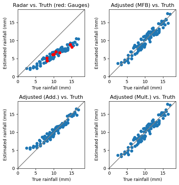
[12]:
# Open figure
fig = plt.figure(figsize=(6, 6))

# Scatter plot radar vs. observations
ax = fig.add_subplot(221, aspect="equal")
scatterplot(truth, radar, "Radar vs. Truth (red: Gauges)")
plt.plot(obs, radar[obs_ix], linestyle="None", marker="o", color="red")

# Adjusted (MFB) vs. radar (for control purposes)
ax = fig.add_subplot(222, aspect="equal")
scatterplot(truth, mfbadjusted, "Adjusted (MFB) vs. Truth")

# Adjusted (Add) vs. radar (for control purposes)
ax = fig.add_subplot(223, aspect="equal")
scatterplot(truth, addadjusted, "Adjusted (Add.) vs. Truth")

# Adjusted (Mult.) vs. radar (for control purposes)
ax = fig.add_subplot(224, aspect="equal")
scatterplot(truth, multadjusted, "Adjusted (Mult.) vs. Truth")

plt.tight_layout()