Interpolate data from polar to cartesian coordinates#
The \(\omega radlib\) wradlib.ipol module implements several interpolator schemes, many of them based on scipy.spatial.cKDTree class. In this notebook its shown how they are applied to xarray.Dataset or xarray.DataArray.
import numpy as np
import matplotlib.pyplot as plt
import wradlib as wrl
import wradlib_data
import warnings
import xarray as xr
import cmweather

warnings.filterwarnings("ignore")
/home/docs/checkouts/readthedocs.org/user_builds/wradlib/conda/latest/lib/python3.13/site-packages/tqdm/auto.py:21: TqdmWarning: IProgress not found. Please update jupyter and ipywidgets. See https://ipywidgets.readthedocs.io/en/stable/user_install.html
  from .autonotebook import tqdm as notebook_tqdm
Import polar and cartesian data#
filename1 = wradlib_data.DATASETS.fetch("geo/bonn_new.tif")
dem_bonn = xr.open_dataset(filename1, engine="rasterio")

filename2 = wradlib_data.DATASETS.fetch("hdf5/2014-08-10--182000.ppi.mvol")
swp = xr.open_dataset(filename2, engine="gamic", group="sweep_0")
Preprocess polar data#
In order to be on the same coordinates, we georeference the radar sweep coordinates accordingly.
swp = swp.wrl.georef.georeference(crs=dem_bonn.spatial_ref)
swp = swp.set_coords("sweep_mode")
swp = swp.isel(range=slice(0, 100))
display(swp)
<xarray.Dataset> Size: 3MB
Dimensions:            (azimuth: 360, range: 100)
Coordinates: (12/15)
  * azimuth            (azimuth) float64 3kB 0.5054 1.522 2.527 ... 358.5 359.5
    elevation          (azimuth) float64 3kB 1.505 1.505 1.505 ... 1.505 1.505
    time               (azimuth) datetime64[ns] 3kB ...
  * range              (range) float32 400B 50.0 150.0 ... 9.85e+03 9.95e+03
    x                  (azimuth, range) float64 288kB 7.072 7.072 ... 7.07 7.07
    y                  (azimuth, range) float64 288kB 50.73 50.73 ... 50.82
    ...                 ...
    bins               (azimuth, range) float32 144kB 50.0 150.0 ... 9.95e+03
    sweep_mode         <U20 80B 'azimuth_surveillance'
    longitude          float64 8B 7.072
    latitude           float64 8B 50.73
    altitude           float64 8B 99.5
    crs_wkt            int64 8B 0
Data variables: (12/17)
    KDP                (azimuth, range) float32 144kB ...
    PHIDP              (azimuth, range) float32 144kB ...
    DBZH               (azimuth, range) float32 144kB ...
    DBZV               (azimuth, range) float32 144kB ...
    RHOHV              (azimuth, range) float32 144kB ...
    DBTH               (azimuth, range) float32 144kB ...
    ...                 ...
    ZDR                (azimuth, range) float32 144kB ...
    sweep_number       int64 8B ...
    prt_mode           <U7 28B ...
    follow_mode        <U7 28B ...
    sweep_fixed_angle  float64 8B ...
    nyquist_velocity   object 8B ...
Attributes:
    source:       gamic
pulse_width: 2Preprocess cartesian data#
First, inspect the data set a little.
display(dem_bonn)
<xarray.Dataset> Size: 69MB
Dimensions:      (band: 1, x: 4800, y: 3600)
Coordinates:
  * band         (band) int64 8B 1
  * x            (x) float64 38kB 5.0 5.001 5.002 5.003 ... 8.998 8.999 9.0
  * y            (y) float64 29kB 52.0 52.0 52.0 52.0 ... 49.0 49.0 49.0 49.0
    spatial_ref  int64 8B ...
Data variables:
band_data (band, y, x) float32 69MB ...Extract dem_bonn band and crop grid.
band = (
    dem_bonn
    .wrl.util.crop(swp, pad=0)
    .isel(band=0)["band_data"]
)
display(band)
<xarray.DataArray 'band_data' (y: 215, x: 338)> Size: 291kB
[72670 values with dtype=float32]
Coordinates:
  * y            (y) float64 2kB 50.82 50.82 50.82 50.82 ... 50.64 50.64 50.64
  * x            (x) float64 3kB 6.931 6.932 6.933 6.934 ... 7.21 7.211 7.212
    band         int64 8B 1
    spatial_ref  int64 8B ...
Attributes:
AREA_OR_POINT: AreaNearest neighbour interpolation#
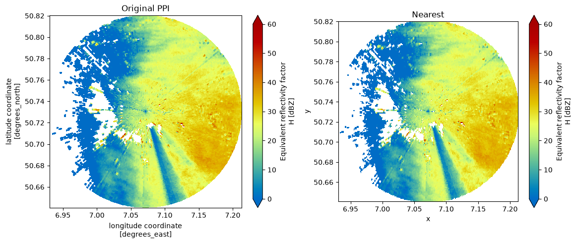
For details see \(\omega radlib\)’s central interpolation API entrypoint wradlib.ipol.IpolMethods.interpolate.
Please check with scipy.spatial.cKDTree for kwargs for tree initialization and scipy.spatial.cKDTree.query for kwargs for querying the tree.
band_xy = band.chunk()
nearest = swp.wrl.ipol.interpolate(band_xy, method="nearest")
display(nearest)
<xarray.Dataset> Size: 3MB
Dimensions:            (y: 215, x: 338)
Coordinates:
  * y                  (y) float64 2kB 50.82 50.82 50.82 ... 50.64 50.64 50.64
  * x                  (x) float64 3kB 6.931 6.932 6.933 ... 7.21 7.211 7.212
    sweep_mode         <U20 80B 'azimuth_surveillance'
    longitude          float64 8B 7.072
    latitude           float64 8B 50.73
    altitude           float64 8B 99.5
    crs_wkt            int64 8B 0
    band               int64 8B 1
    spatial_ref        int64 8B 0
Data variables: (12/17)
    KDP                (y, x) float32 291kB nan nan nan nan ... nan nan nan nan
    PHIDP              (y, x) float32 291kB nan nan nan nan ... nan nan nan nan
    DBZH               (y, x) float32 291kB nan nan nan nan ... nan nan nan nan
    DBZV               (y, x) float32 291kB nan nan nan nan ... nan nan nan nan
    RHOHV              (y, x) float32 291kB nan nan nan nan ... nan nan nan nan
    DBTH               (y, x) float32 291kB nan nan nan nan ... nan nan nan nan
    ...                 ...
    ZDR                (y, x) float32 291kB nan nan nan nan ... nan nan nan nan
    sweep_number       int64 8B ...
    prt_mode           <U7 28B ...
    follow_mode        <U7 28B ...
    sweep_fixed_angle  float64 8B ...
nyquist_velocity object 8B ...fig, (ax1, ax2) = plt.subplots(1, 2, figsize=(12, 5))
cmap = "HomeyerRainbow"
vmin, vmax = 0.0, 60.0
pm = swp.DBZH.wrl.vis.plot(ax=ax1, cmap=cmap, vmin=vmin, vmax=vmax)
ax1.set_title("Original PPI")
pm = nearest.DBZH.plot(ax=ax2, cmap=cmap, vmin=vmin, vmax=vmax)
ax2.set_aspect(nearest.wrl.util.aspect())
ax2.set_title("Nearest")
plt.tight_layout()
Inverse distance#
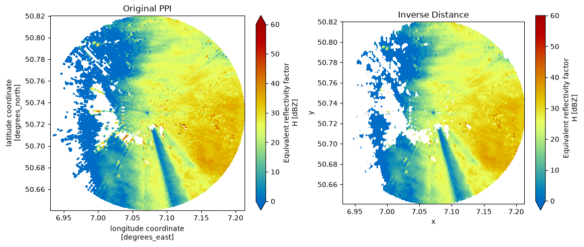
For details see \(\omega radlib\)’s central interpolation API entrypoint wradlib.ipol.IpolMethods.interpolate.
Please check with scipy.spatial.cKDTree for kwargs for tree initialization and scipy.spatial.cKDTree.query for kwargs for querying the tree.
band_xy = band.chunk()
inverse_distance = swp.wrl.ipol.interpolate(band_xy, method="inverse_distance", k=4, idw_p=2)
display(inverse_distance)
<xarray.Dataset> Size: 7MB
Dimensions:            (y: 215, x: 338)
Coordinates:
  * y                  (y) float64 2kB 50.82 50.82 50.82 ... 50.64 50.64 50.64
  * x                  (x) float64 3kB 6.931 6.932 6.933 ... 7.21 7.211 7.212
    sweep_mode         <U20 80B 'azimuth_surveillance'
    longitude          float64 8B 7.072
    latitude           float64 8B 50.73
    altitude           float64 8B 99.5
    crs_wkt            int64 8B 0
    band               int64 8B 1
    spatial_ref        int64 8B 0
Data variables: (12/17)
    KDP                (y, x) float64 581kB nan nan nan nan ... nan nan nan nan
    PHIDP              (y, x) float64 581kB nan nan nan nan ... nan nan nan nan
    DBZH               (y, x) float64 581kB nan nan nan nan ... nan nan nan nan
    DBZV               (y, x) float64 581kB nan nan nan nan ... nan nan nan nan
    RHOHV              (y, x) float64 581kB nan nan nan nan ... nan nan nan nan
    DBTH               (y, x) float64 581kB nan nan nan nan ... nan nan nan nan
    ...                 ...
    ZDR                (y, x) float64 581kB nan nan nan nan ... nan nan nan nan
    sweep_number       int64 8B ...
    prt_mode           <U7 28B ...
    follow_mode        <U7 28B ...
    sweep_fixed_angle  float64 8B ...
nyquist_velocity object 8B ...fig, (ax1, ax2) = plt.subplots(1, 2, figsize=(12, 5))
cmap = "HomeyerRainbow"
vmin, vmax = 0.0, 60.0
pm = swp.DBZH.wrl.vis.plot(ax=ax1, cmap=cmap, vmin=vmin, vmax=vmax)
ax1.set_title("Original PPI")
pm = inverse_distance.DBZH.plot(ax=ax2, cmap=cmap, vmin=vmin, vmax=vmax)
ax2.set_aspect(inverse_distance.wrl.util.aspect())
ax2.set_title("Inverse Distance")
plt.tight_layout()
Precompute KDTree dataset#
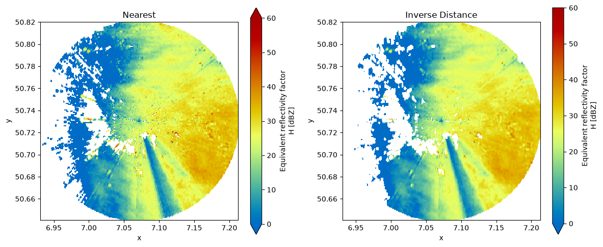
In the above examples the KDTree is computed and queried within the function. If your geometry is fixed you can precompute the KDTree and use it in subsequent computations.
Please check with scipy.spatial.cKDTree for kwargs for tree initialization and scipy.spatial.cKDTree.query for kwargs for querying the tree.
band_xy = band.chunk()
mapping = swp.wrl.ipol.get_mapping(band_xy, k=4)
display(mapping)
<xarray.Dataset> Size: 5MB
Dimensions:      (x: 338, y: 215, k: 4)
Coordinates:
  * x            (x) float64 3kB 6.931 6.932 6.933 6.934 ... 7.21 7.211 7.212
  * y            (y) float64 2kB 50.82 50.82 50.82 50.82 ... 50.64 50.64 50.64
  * k            (k) int64 32B 0 1 2 3
    band         int64 8B 1
    spatial_ref  int64 8B ...
Data variables:
    ix           (k, x, y) int64 2MB 30799 30799 30799 ... 12599 12599 12599
    dists        (k, x, y) float64 2MB 0.04491 0.04427 ... 0.0447 0.04538
Attributes:
    source:        wradlib
    model:         kdtree
    tree_kwargs:   {'balanced_tree': False}
query_kwargs: {'k': 4, 'workers': -1}band_xy = band.chunk()
nearest = swp.wrl.ipol.interpolate(mapping, method="nearest")
inverse_distance = swp.wrl.ipol.interpolate(mapping, method="inverse_distance", idw_p=2)
fig, (ax1, ax2) = plt.subplots(1, 2, figsize=(12, 5))
cmap = "HomeyerRainbow"
vmin, vmax = 0.0, 60.0

pm = nearest.DBZH.plot(ax=ax1, cmap=cmap, vmin=vmin, vmax=vmax)
ax1.set_aspect(nearest.wrl.util.aspect())
ax1.set_title("Nearest")

pm = inverse_distance.DBZH.plot(ax=ax2, cmap=cmap, vmin=vmin, vmax=vmax)
ax2.set_aspect(inverse_distance.wrl.util.aspect())
ax2.set_title("Inverse Distance")

plt.tight_layout()