System Differential Phase \(\Phi_{DP}^{sys}\)#
import warnings

from IPython.display import display

warnings.filterwarnings("ignore")
Correct retrieval of \(\Phi_{DP}^{sys}\) (Offset) is crucial for correct processing of further derivations. Normally \(\Phi_{DP}^{sys}\) is more or less constant. It can have azimuthal/elevational deviations, eg. depending on the antenna near field.
Retrieval of \(\Phi_{DP}^{sys}\) is sometimes tedious, due to the contamination of the signal with clutter and other artifacts.
Import Section#
import matplotlib.pyplot as plt
import numpy as np
import xarray as xr
import wradlib as wrl
import open_radar_data
Open Dataset#
We use a dataset from Surgavere Radar, Estonia.
filename = open_radar_data.DATASETS.fetch("SUR.202506091000.VOL.h5")
swp = xr.open_dataset(filename, engine="odim", group="sweep_0").set_coords("sweep_mode").wrl.georef.georeference()
display(swp)
Downloading file 'SUR.202506091000.VOL.h5' from 'https://github.com/openradar/open-radar-data/raw/main/data/SUR.202506091000.VOL.h5' to '/home/docs/.cache/open-radar-data'.
<xarray.Dataset> Size: 43MB
Dimensions:            (azimuth: 360, range: 833)
Coordinates: (12/15)
  * azimuth            (azimuth) float64 3kB 0.02747 1.038 2.057 ... 358.1 359.1
    elevation          (azimuth) float64 3kB 0.5 0.5 0.5 0.5 ... 0.5 0.5 0.5 0.5
    time               (azimuth) datetime64[ns] 3kB ...
  * range              (range) float32 3kB 150.0 450.0 ... 2.494e+05 2.498e+05
    x                  (azimuth, range) float64 2MB 0.0719 0.2157 ... -4.068e+03
    y                  (azimuth, range) float64 2MB 150.0 450.0 ... 2.496e+05
    ...                 ...
    bins               (azimuth, range) float32 1MB 150.0 450.0 ... 2.498e+05
    sweep_mode         <U20 80B 'azimuth_surveillance'
    longitude          float64 8B 25.52
    latitude           float64 8B 58.48
    altitude           float64 8B 157.0
    crs_wkt            int64 8B 0
Data variables: (12/18)
    TH                 (azimuth, range) float64 2MB ...
    HCLASS             (azimuth, range) float32 1MB ...
    SNR                (azimuth, range) float64 2MB ...
    PMI                (azimuth, range) float64 2MB ...
    CSP                (azimuth, range) float64 2MB ...
    DBZH               (azimuth, range) float64 2MB ...
    ...                 ...
    PHIDP              (azimuth, range) float64 2MB ...
    sweep_number       int64 8B ...
    prt_mode           <U7 28B ...
    follow_mode        <U7 28B ...
    sweep_fixed_angle  float64 8B ...
    nyquist_velocity   float64 8B ...
Attributes:
Conventions: ODIM_H5/V2_2Inspect Dataset#
display(swp)
<xarray.Dataset> Size: 43MB
Dimensions:            (azimuth: 360, range: 833)
Coordinates: (12/15)
  * azimuth            (azimuth) float64 3kB 0.02747 1.038 2.057 ... 358.1 359.1
    elevation          (azimuth) float64 3kB 0.5 0.5 0.5 0.5 ... 0.5 0.5 0.5 0.5
    time               (azimuth) datetime64[ns] 3kB ...
  * range              (range) float32 3kB 150.0 450.0 ... 2.494e+05 2.498e+05
    x                  (azimuth, range) float64 2MB 0.0719 0.2157 ... -4.068e+03
    y                  (azimuth, range) float64 2MB 150.0 450.0 ... 2.496e+05
    ...                 ...
    bins               (azimuth, range) float32 1MB 150.0 450.0 ... 2.498e+05
    sweep_mode         <U20 80B 'azimuth_surveillance'
    longitude          float64 8B 25.52
    latitude           float64 8B 58.48
    altitude           float64 8B 157.0
    crs_wkt            int64 8B 0
Data variables: (12/18)
    TH                 (azimuth, range) float64 2MB ...
    HCLASS             (azimuth, range) float32 1MB ...
    SNR                (azimuth, range) float64 2MB ...
    PMI                (azimuth, range) float64 2MB ...
    CSP                (azimuth, range) float64 2MB ...
    DBZH               (azimuth, range) float64 2MB ...
    ...                 ...
    PHIDP              (azimuth, range) float64 2MB ...
    sweep_number       int64 8B ...
    prt_mode           <U7 28B ...
    follow_mode        <U7 28B ...
    sweep_fixed_angle  float64 8B ...
    nyquist_velocity   float64 8B ...
Attributes: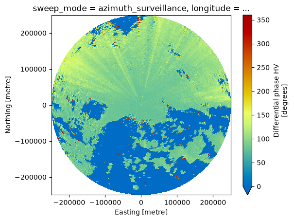
Conventions: ODIM_H5/V2_2swp.PHIDP.wrl.vis.plot(vmin=0, vmax=360)
<matplotlib.collections.QuadMesh at 0x7448747fa7b0>
System Differential Phase \(\Phi_{DP}^{sys}\) via first precipitating bins#
This is a most common algorithm. But there are several approaches. All use common \(\rho_{HV}\) filtering or other means of reducing unwanted artifacts in \(\Phi_{DP}^{sys}\).
N consecutive radar bins with \(\rho_{HV}\) > threshold
maximum number of valid bins in a N-size window
first N valid bins (not necessarily consecutive)
Mask source data#
Essential pre-step masking unwanted signal.
phimask = swp.PHIDP.where(swp.RHOHV >= 0.9)
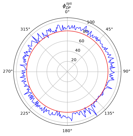
N consecutive valid radar bins#
It finds the first N consecutive precipitating bins per each ray
and uses the median of these values to determine the offset per ray.
If there are only a few of those radials (<30) per sweep we’ll use a default value from a previous sweep
Sort the median values from 2. and calculate the median from the smallest 30 (default). That value is considered \(\Phi_{DP}^{sys}\).
See also
phisys_block = phimask.wrl.dp.system_phidp_block(rng=2000.)
display(phisys_block)
<xarray.Dataset> Size: 17kB
Dimensions:      (azimuth: 360)
Coordinates:
  * azimuth      (azimuth) float64 3kB 0.02747 1.038 2.057 ... 357.1 358.1 359.1
    elevation    (azimuth) float64 3kB 0.5 0.5 0.5 0.5 0.5 ... 0.5 0.5 0.5 0.5
    time         (azimuth) datetime64[ns] 3kB 2025-06-09T10:00:24.080583680 ....
    sweep_mode   <U20 80B 'azimuth_surveillance'
    longitude    float64 8B 25.52
    latitude     float64 8B 58.48
    altitude     float64 8B 157.0
    crs_wkt      int64 8B 0
Data variables:
    sysphi_ray   (azimuth) float64 3kB 91.9 94.72 95.22 ... 94.71 83.42 89.25
    sysphi       float64 8B 79.48
    start_range  (azimuth) float32 1kB 750.0 150.0 150.0 ... 1.65e+03 750.0
    stop_range   (azimuth) float32 1kB 2.55e+03 1.95e+03 ... 3.45e+03 2.55e+03
    valid_bins   (azimuth) int64 3kB 7 7 7 7 7 7 7 7 7 7 ... 7 7 7 7 7 7 7 7 7 7
Attributes:
    _Undetect:      0.0
    units:          degrees
    standard_name:  radar_differential_phase_hv
long_name: Differential phase HVfig, (ax1, ax2) = plt.subplots(2, 1, figsize=(10, 10), sharex=True)
phisys_block.start_range.plot(ax=ax1, lw=0.8, c="k")
phisys_block.stop_range.plot(ax=ax1, lw=0.8, c="k")
phimask.plot(ax=ax1, x="azimuth", y="range", cmap="turbo", vmin=0, vmax=140)
ax1.set_title(rf"$\phi_{{DP}}^{{sys}}$ - {phisys_block.valid_bins[0].values} consecutive valid radar bins")
phisys_block.start_range.plot(ax=ax2, lw=0.8, c="k")
phisys_block.stop_range.plot(ax=ax2, lw=0.8, c="k")
phimask.plot(ax=ax2, x="azimuth", y="range", cmap="turbo", vmin=0, vmax=140)
ax2.set_title(rf"$\phi_{{DP}}^{{sys}}$ - zoom")
ax2.set_ylim(0, 15e3)
display(phisys_block.sysphi)
fig.tight_layout()
<xarray.DataArray 'sysphi' ()> Size: 8B
array(79.47752312)
Coordinates:
    sweep_mode  <U20 80B 'azimuth_surveillance'
    longitude   float64 8B 25.52
    latitude    float64 8B 58.48
    altitude    float64 8B 157.0
    crs_wkt     int64 8B 0
Attributes:
    _Undetect:      0.0
    units:          degrees
    standard_name:  radar_differential_phase_hv
    long_name:      Differential phase HV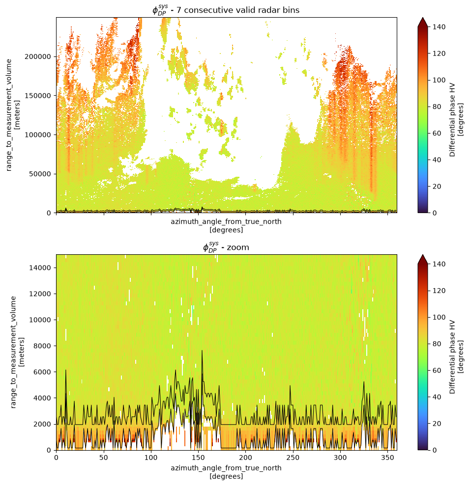
fig = plt.figure()
ax = fig.add_subplot(projection="polar")
# set the lable go clockwise and start from the top
ax.set_theta_zero_location("N")
# clockwise
ax.set_theta_direction(-1)

theta = np.linspace(0, 2 * np.pi, num=phisys_block.dims["azimuth"], endpoint=False)
ax.plot(theta, phisys_block.sysphi_ray, color="b", linewidth=1)
ax.plot(theta, np.ones_like(theta)*phisys_block.sysphi.values, color="r", linewidth=1)
_ = ax.set_title(rf"$\phi_{{DP}}^{{sys}}$")
maximum number of valid radar bins in N-sized window#
Calculate the number of valid bins for a window of size N along the ray
find the position where this valid bin number has it’s maximum along the ray
and uses the median of these values to determine the offset per ray.
a) Sort the median values from 3. and calculate the median from the smallest 30. That value is considered \(\Phi_{DP}^{sys}\). b) Calculate the median from 3. That value is considered system PhiDP.
See also
phisys_window = phimask.wrl.dp.system_phidp_window(2000.)
display(phisys_window)
<xarray.Dataset> Size: 17kB
Dimensions:      (azimuth: 360)
Coordinates:
  * azimuth      (azimuth) float64 3kB 0.02747 1.038 2.057 ... 357.1 358.1 359.1
    elevation    (azimuth) float64 3kB 0.5 0.5 0.5 0.5 0.5 ... 0.5 0.5 0.5 0.5
    time         (azimuth) datetime64[ns] 3kB 2025-06-09T10:00:24.080583680 ....
    sweep_mode   <U20 80B 'azimuth_surveillance'
    longitude    float64 8B 25.52
    latitude     float64 8B 58.48
    altitude     float64 8B 157.0
    crs_wkt      int64 8B 0
Data variables:
    sysphi_ray   (azimuth) float64 3kB 91.9 94.72 95.22 ... 94.71 83.42 89.25
    sysphi       float64 8B 79.48
    start_range  (azimuth) float32 1kB 750.0 150.0 150.0 ... 1.65e+03 750.0
    stop_range   (azimuth) float32 1kB 2.55e+03 1.95e+03 ... 3.45e+03 2.55e+03
    valid_bins   (azimuth) float64 3kB 7.0 7.0 7.0 7.0 7.0 ... 7.0 7.0 7.0 7.0
Attributes:
    _Undetect:      0.0
    units:          degrees
    standard_name:  radar_differential_phase_hv
long_name: Differential phase HVfig, (ax1, ax2) = plt.subplots(2, 1, figsize=(10, 10), sharex=True)
phisys_window.start_range.plot(ax=ax1, lw=0.8, c="k")
phisys_window.stop_range.plot(ax=ax1, lw=0.8, c="k")
phimask.plot(ax=ax1, x="azimuth", y="range", cmap="turbo", vmin=0, vmax=140)
ax1.set_title(rf"$\phi_{{DP}}^{{sys}}$ - {phisys_window.valid_bins[0].values} valid radar bins")
phisys_window.start_range.plot(ax=ax2, lw=0.8, c="k")
phisys_window.stop_range.plot(ax=ax2, lw=0.8, c="k")
phimask.plot(ax=ax2, x="azimuth", y="range", cmap="turbo", vmin=0, vmax=140)
ax2.set_title(rf"$\phi_{{DP}}^{{sys}}$ - zoom")
ax2.set_ylim(0, 15e3)
display(phisys_window.sysphi)
fig.tight_layout()
<xarray.DataArray 'sysphi' ()> Size: 8B
array(79.47752312)
Coordinates:
    sweep_mode  <U20 80B 'azimuth_surveillance'
    longitude   float64 8B 25.52
    latitude    float64 8B 58.48
    altitude    float64 8B 157.0
    crs_wkt     int64 8B 0
Attributes:
    _Undetect:      0.0
    units:          degrees
    standard_name:  radar_differential_phase_hv
    long_name:      Differential phase HV
fig = plt.figure()
ax = fig.add_subplot(projection="polar")
# set the lable go clockwise and start from the top
ax.set_theta_zero_location("N")
# clockwise
ax.set_theta_direction(-1)

theta = np.linspace(0, 2 * np.pi, num=phisys_window.dims["azimuth"], endpoint=False)
ax.plot(theta, phisys_window.sysphi_ray, color="b", linewidth=1)
ax.plot(theta, np.ones_like(theta)*phisys_window.sysphi.values, color="r", linewidth=1)
_ = ax.set_title(rf"$\phi_{{DP}}^{{sys}}$")
first N valid bins#
get the first N valid bins per each ray
calculate median from these values
a) Sort the median values from 2. and calculate the median from the smallest 30. That value is considered \(\Phi_{DP}^{sys}\). b) Calculate the median from 2. That value is considered system PhiDP.
See also
phisys_first = phimask.wrl.dp.system_phidp_first(11)
display(phisys_first)
<xarray.Dataset> Size: 17kB
Dimensions:      (azimuth: 360)
Coordinates:
  * azimuth      (azimuth) float64 3kB 0.02747 1.038 2.057 ... 357.1 358.1 359.1
    elevation    (azimuth) float64 3kB 0.5 0.5 0.5 0.5 0.5 ... 0.5 0.5 0.5 0.5
    time         (azimuth) datetime64[ns] 3kB 2025-06-09T10:00:24.080583680 ....
    sweep_mode   <U20 80B 'azimuth_surveillance'
    longitude    float64 8B 25.52
    latitude     float64 8B 58.48
    altitude     float64 8B 157.0
    crs_wkt      int64 8B 0
Data variables:
    sysphi_ray   (azimuth) float64 3kB 86.34 89.42 89.95 ... 86.58 82.96 85.08
    sysphi       float64 8B 79.65
    start_range  (azimuth) float32 1kB 750.0 150.0 150.0 ... 1.65e+03 750.0
    stop_range   (azimuth) float32 1kB 3.75e+03 3.15e+03 ... 4.65e+03 3.75e+03
    valid_bins   (azimuth) int64 3kB 11 11 11 11 11 11 11 ... 11 11 11 11 11 11
Attributes:
    _Undetect:      0.0
    units:          degrees
    standard_name:  radar_differential_phase_hv
long_name: Differential phase HVfig, (ax1, ax2) = plt.subplots(2, 1, figsize=(10, 10), sharex=True)
phisys_first.start_range.plot(ax=ax1, lw=0.8, c="k")
phisys_first.stop_range.plot(ax=ax1, lw=0.8, c="k")
phimask.plot(ax=ax1, x="azimuth", y="range", cmap="turbo", vmin=0, vmax=140)
ax1.set_title(rf"$\phi_{{DP}}^{{sys}}$ - {phisys_first.valid_bins[0].values} valid radar bins")
phisys_first.start_range.plot(ax=ax2, lw=0.8, c="k")
phisys_first.stop_range.plot(ax=ax2, lw=0.8, c="k")
phimask.plot(ax=ax2, x="azimuth", y="range", cmap="turbo", vmin=0, vmax=140)
ax2.set_title(rf"$\phi_{{DP}}^{{sys}}$ - zoom")
ax2.set_ylim(0, 15e3)
display(phisys_first.sysphi)
fig.tight_layout()
<xarray.DataArray 'sysphi' ()> Size: 8B
array(79.6478164)
Coordinates:
    sweep_mode  <U20 80B 'azimuth_surveillance'
    longitude   float64 8B 25.52
    latitude    float64 8B 58.48
    altitude    float64 8B 157.0
    crs_wkt     int64 8B 0
Attributes:
    _Undetect:      0.0
    units:          degrees
    standard_name:  radar_differential_phase_hv
    long_name:      Differential phase HV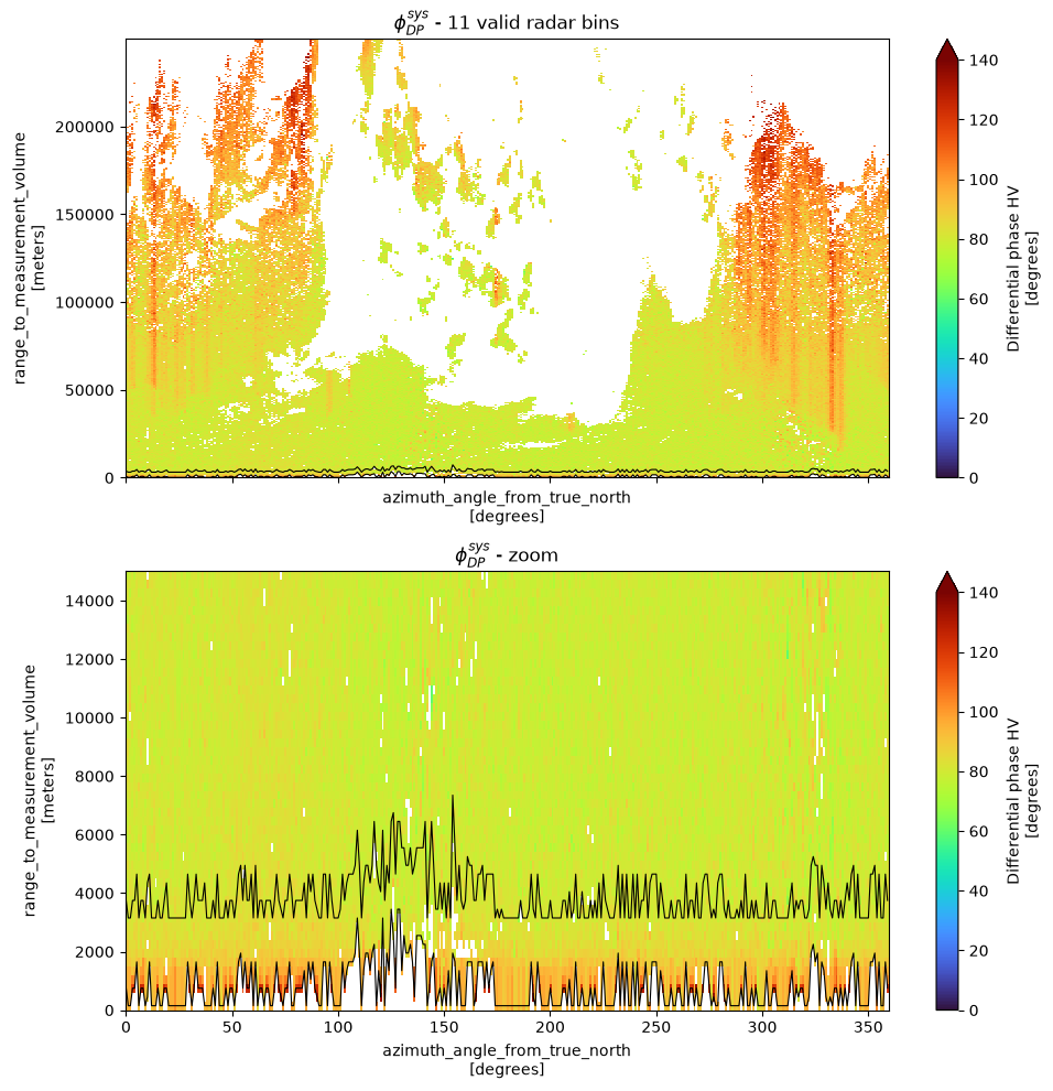
fig = plt.figure()
ax = fig.add_subplot(projection="polar")
# set the lable go clockwise and start from the top
ax.set_theta_zero_location("N")
# clockwise
ax.set_theta_direction(-1)

theta = np.linspace(0, 2 * np.pi, num=phisys_first.dims["azimuth"], endpoint=False)
ax.plot(theta, phisys_first.sysphi_ray, color="b", linewidth=1)
ax.plot(theta, np.ones_like(theta)*phisys_first.sysphi.values, color="r", linewidth=1)
_ = ax.set_title(rf"$\phi_{{DP}}^{{sys}}$")
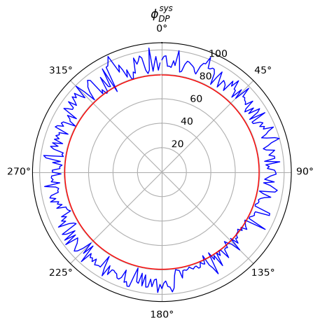
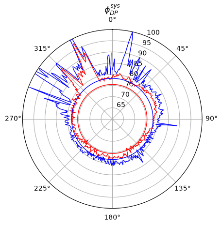
System Differential Phase \(\Phi_{DP}^{sys}\) via phase histogram#
The idea behind is:
\(\Phi_{DP}^{sys}\) is constantly increasing
\(\Phi_{DP}^{sys}\) is inherently noisy
That means, the majority of phase measurements (precipitating bins) should lie around \(\Phi_{DP}^{sys}\). It’s relatively robust since it does not rely on finding precipitating bins in each ray or the like. Nevertheless, taking a pre-filtered phase as input should return similar results.
See also
from xhistogram.xarray import histogram as xhist

hlist = []
phase_res = 0.1
bins = (0, 360, phase_res)
phisys_hist = swp.PHIDP.wrl.dp.system_phidp_hist(bins=bins)
display(phisys_hist)
<xarray.Dataset> Size: 10MB
Dimensions:           (azimuth: 360, bin: 3599)
Coordinates:
  * azimuth           (azimuth) float64 3kB 0.02747 1.038 2.057 ... 358.1 359.1
  * bin               (bin) float64 29kB 0.05 0.15 0.25 ... 359.7 359.8 359.9
Data variables:
    sysphi_hist       (azimuth, bin) int64 10MB 0 0 0 0 0 0 0 ... 0 0 0 0 0 0 0
    sysphi_peak_ray   (azimuth) float64 3kB 82.15 83.75 86.85 ... 79.75 89.55
    sysphi_first_ray  (azimuth) float64 3kB 78.55 79.95 79.25 ... 77.65 78.55
    sysphi_peak       float64 8B 78.15
sysphi_first float64 8B 75.45fig = plt.figure()
ax = fig.add_subplot(projection="polar")
# set the lable go clockwise and start from the top
ax.set_theta_zero_location("N")
# clockwise
ax.set_theta_direction(-1)
theta = np.linspace(0, 2 * np.pi, num=phisys_first.dims["azimuth"], endpoint=False)
ax.plot(theta, phisys_hist.sysphi_peak_ray, color="b", linewidth=1)
ax.plot(theta, phisys_hist.sysphi_first_ray, color="r", linewidth=1)
ax.plot(theta, np.ones_like(theta)*phisys_hist.sysphi_peak.values, color="b", linewidth=1.0)
ax.plot(theta, np.ones_like(theta)*phisys_hist.sysphi_first.values, color="r", linewidth=1.0)
_ = ax.set_title(rf"$\phi_{{DP}}^{{sys}}$")
ax.set_ylim(60, 100)
(60.0, 100.0)
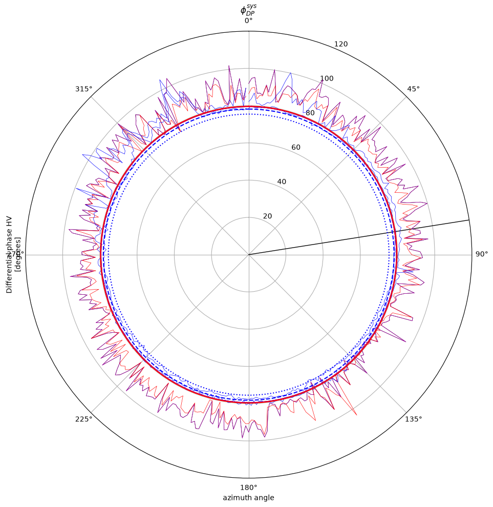
Overview and Diagnostic plots#
add theta in radians to dataset
theta = np.linspace(0, 2 * np.pi, num=360, endpoint=False)
phisys_block = phisys_block.assign_coords(
    theta=(["azimuth"], theta, {"standard_name": "azimuth angle"})
)
phisys_window = phisys_window.assign_coords(
    theta=(["azimuth"], theta, {"standard_name": "azimuth angle"})
)
phisys_first = phisys_first.assign_coords(
    theta=(["azimuth"], theta, {"standard_name": "azimuth angle"})
)
phisys_hist = phisys_hist.assign_coords(
    theta=(["azimuth"], theta, {"standard_name": "azimuth angle"})
)
vmin = 0
vmax = 120
startaz = swp.sortby("time").azimuth[0]

fig = plt.figure(figsize=(10, 10))
ax = fig.add_subplot(projection="polar")
ax.set_theta_zero_location("N")
ax.set_theta_direction(-1)

ax.axvline(np.radians(startaz.values), c="black", lw=1.0)
phisys_block.sysphi_ray.plot(x="theta", c="k", lw=0.5, ax=ax)
phisys_window.sysphi_ray.plot(x="theta", c="m", lw=0.5, ax=ax)
phisys_first.sysphi_ray.plot(x="theta", c="r", lw=0.5, ax=ax)
phisys_hist.sysphi_peak_ray.plot(x="theta", c="b", lw=0.5, ax=ax)
phisys_hist.sysphi_first_ray.plot(x="theta", c="b", lw=0.5, ax=ax)
ax.axhline(phisys_block.sysphi, c="k").get_path()._interpolation_steps = 180
ax.axhline(phisys_window.sysphi, c="m").get_path()._interpolation_steps = 180
ax.axhline(phisys_first.sysphi, c="r").get_path()._interpolation_steps = 180
ax.axhline(phisys_hist.sysphi_peak, c="b", ls="--").get_path()._interpolation_steps = 180
ax.axhline(phisys_hist.sysphi_first, c="b", ls=":").get_path()._interpolation_steps = 180
ax.set_ylim(vmin, vmax)
ax.set_title(rf"$\phi_{{DP}}^{{sys}}$")
plt.tight_layout()