Total Differential Phase Shift \(\Delta \Phi_{DP}\)#
import warnings

from IPython.display import display

warnings.filterwarnings("ignore")
The total differential phase shift, denoted as \(\Delta \Phi_{DP}^{tot}\), is a path-integrated radar variable that represents the accumulated change in differential phase (\(\Phi_{DP}\)) along a radar ray between two range locations.
Unlike reflectivity,\(\Phi_{DP}\) is a propagation phase quantity that increases monotonically with range in precipitation and is largely unaffected by attenuation and calibration biases. This makes it a robust constraint for attenuation and rainfall microphysics retrievals.
In the ZPHI framework, \(\Delta \Phi_{DP}^{tot}\) serves as the key normalization quantity linking local reflectivity structure to integrated propagation effects.
\(\Delta \Phi_{DP}\) represents the net phase shift induced by hydrometeors along a selected radar path segment:
\(\begin{equation} \Delta\Phi_{DP} = \Phi_{DP}(r_2) - \Phi_{DP}(r_1) \tag{1} \end{equation}\)
where:
\(r_1\) - start of the selected valid radar interval
\(r_2\) - end of the selected valid radar interval
This interval is not fixed a priori, but is determined dynamically based on data quality and spatial continuity.
Import Section#
import matplotlib.pyplot as plt
import numpy as np
import xarray as xr
import wradlib as wrl
import wradlib_data
import open_radar_data
Open Dataset#
We use a dataset from BoXPol, Germany.
fname = wradlib_data.DATASETS.fetch("hdf5/2014-08-10--182000.ppi.mvol")
with xr.open_dataset(fname, engine="gamic", group="sweep_0") as swp:
    swp = swp.set_coords("sweep_mode").wrl.georef.georeference()
Inspect Dataset#
display(swp)
<xarray.Dataset> Size: 33MB
Dimensions:            (azimuth: 360, range: 1000)
Coordinates: (12/15)
  * azimuth            (azimuth) float64 3kB 0.5054 1.522 2.527 ... 358.5 359.5
    elevation          (azimuth) float64 3kB 1.505 1.505 1.505 ... 1.505 1.505
    time               (azimuth) datetime64[ns] 3kB ...
  * range              (range) float32 4kB 50.0 150.0 ... 9.985e+04 9.995e+04
    x                  (azimuth, range) float64 3MB 0.4409 1.323 ... -866.6
    y                  (azimuth, range) float64 3MB 49.98 149.9 ... 9.988e+04
    ...                 ...
    bins               (azimuth, range) float32 1MB 50.0 150.0 ... 9.995e+04
    sweep_mode         <U20 80B 'azimuth_surveillance'
    longitude          float64 8B 7.072
    latitude           float64 8B 50.73
    altitude           float64 8B 99.5
    crs_wkt            int64 8B 0
Data variables: (12/17)
    KDP                (azimuth, range) float32 1MB ...
    PHIDP              (azimuth, range) float32 1MB ...
    DBZH               (azimuth, range) float32 1MB ...
    DBZV               (azimuth, range) float32 1MB ...
    RHOHV              (azimuth, range) float32 1MB ...
    DBTH               (azimuth, range) float32 1MB ...
    ...                 ...
    ZDR                (azimuth, range) float32 1MB ...
    sweep_number       int64 8B ...
    prt_mode           <U7 28B ...
    follow_mode        <U7 28B ...
    sweep_fixed_angle  float64 8B ...
    nyquist_velocity   object 8B ...
Attributes:
    source:       gamic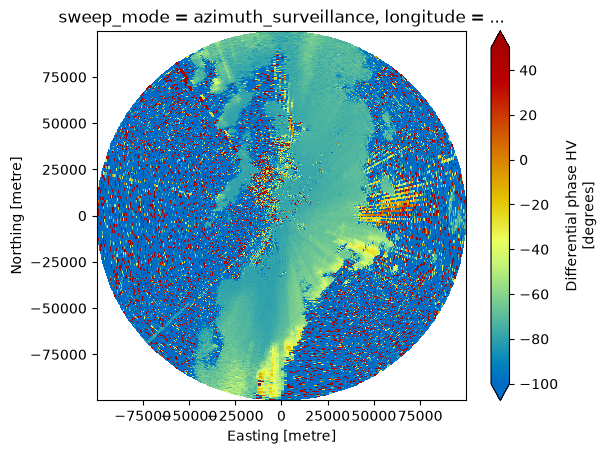
pulse_width: 2swp.PHIDP.wrl.vis.plot(vmin=-100, vmax=50)
<matplotlib.collections.QuadMesh at 0x7e16ce646900>
Total Differential Phase Shift \(\Delta \Phi_{DP}^{tot}\)#
This algorithm is described in detail in [Testud et al., 2000], [Ryzhkov et al., 2014], and [Diederich et al., 2015].
Before computing \(\Delta \Phi_{DP}\), a physically meaningful segment of the radar ray is identified:
invalid or missing observations are masked
a sliding window is used to estimate local data density
the “densest” contiguous region of valid \(\Phi_{DP}\) is selected
This ensures that \(\Delta \Phi_{DP}^{tot}\) is computed only where phase information is reliable.
Mask source data#
Essential pre-step masking unwanted signal.
mask = swp.RHOHV >= 0.9
phimask = swp.PHIDP.where(mask)
dbzmask = swp.DBZH.where(mask)
Estimate ray-based location and values of start and stop window#
We choose 2000m window for estimation of start and stop values.
See also
dphi = phimask.wrl.dp.delta_phidp(rng=2000.)
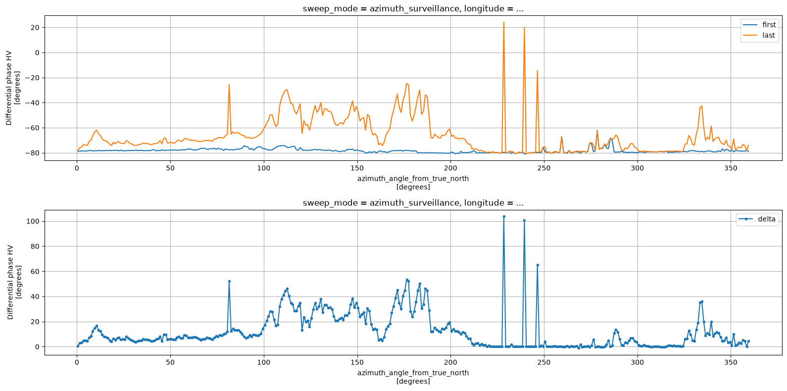
Overview in Cartesian Domain#
fig, (ax1, ax2) = plt.subplots(2, 1, figsize=(16, 8))
dphi.first.plot(label="first", ax=ax1)
dphi.last.plot(label="last", ax=ax1)
ax1.grid()
ax1.legend()
dphi.dphi.plot(ls="-", marker=".", label="delta", ax=ax2)
ax2.grid()
ax2.legend()
plt.tight_layout()
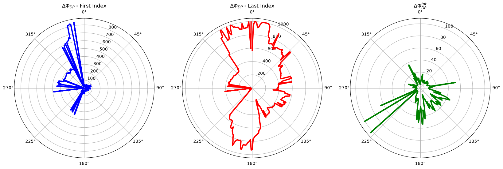
Overview in Polar Domain#
fig = plt.figure(figsize=(20, 14))
ax1 = plt.subplot(231, projection="polar")
ax2 = plt.subplot(232, projection="polar")
ax3 = plt.subplot(233, projection="polar")
# set the lable go clockwise and start from the top
ax1.set_theta_zero_location("N")
ax2.set_theta_zero_location("N")
ax3.set_theta_zero_location("N")
# clockwise
ax1.set_theta_direction(-1)
ax2.set_theta_direction(-1)
ax3.set_theta_direction(-1)

theta = np.linspace(0, 2 * np.pi, num=360, endpoint=False)
ax1.plot(theta, dphi.first_idx, color="b", linewidth=3)
_ = ax1.set_title(r"$\Delta \Phi_{DP}$ - First Index")
ax2.plot(theta, dphi.last_idx, color="r", linewidth=3)
_ = ax2.set_title(r"$\Delta \Phi_{DP}$ - Last Index")
ax3.plot(theta, dphi.dphi, color="g", linewidth=3)
_ = ax3.set_title(r"$\Delta \Phi_{DP}^{tot}$")
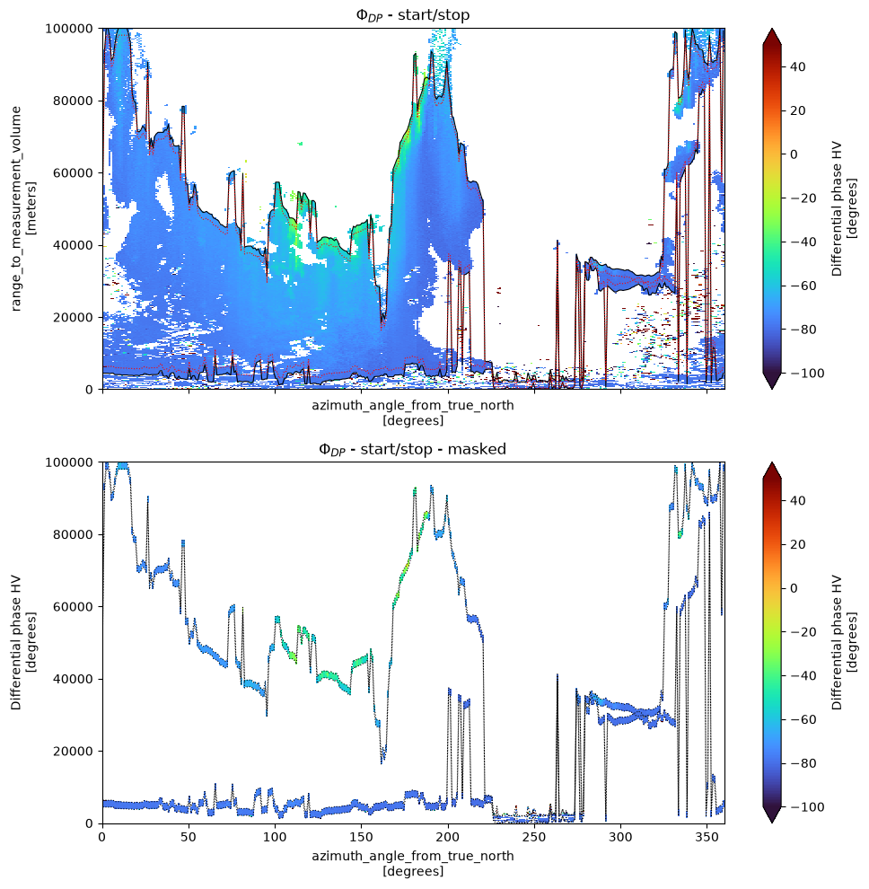
Overview of first and last segments#
fig, (ax1, ax2) = plt.subplots(2, 1, figsize=(10, 10), sharex=True)
dphi.start_range.plot(ax=ax1, lw=0.8, c="k")
(dphi.start_range + dphi.center_span).plot(ax=ax1, lw=0.8, c="r", ls=":")
dphi.stop_range.plot(ax=ax1, lw=0.8, c="k")
(dphi.stop_range - dphi.center_span).plot(ax=ax1, lw=0.8, c="r", ls=":")
phimask.plot(ax=ax1, x="azimuth", y="range", cmap="turbo", vmin=-100, vmax=50)
ax1.set_title(r"$\Phi_{DP}$ - start/stop")

phimask2 = phimask.where(((phimask.range >= dphi.start_range) & (phimask.range <= dphi.start_range + dphi.center_span)) |
                         ((phimask.range >= dphi.stop_range - dphi.center_span) & (phimask.range <= dphi.stop_range)))
phimask2.plot(ax=ax2, x="azimuth", y="range", cmap="turbo", vmin=-100, vmax=50)
dphi.start_range.plot(ax=ax2, lw=0.8, c="k", ls=":")
(dphi.start_range + dphi.center_span).plot(ax=ax2, lw=0.8, c="k", ls=":")
dphi.stop_range.plot(ax=ax2, lw=0.8, c="k", ls=":")
(dphi.stop_range - dphi.center_span).plot(ax=ax2, lw=0.8, c="k", ls=":")
ax2.set_title(r"$\Phi_{DP}$ - start/stop - masked")
fig.tight_layout()