Differential Phase#
In this notebook differential phase \(\Phi_{DP}\) processing is highlighted. This includes phase unfolding as well as derivation of specific differential phase \(K_{DP}\).
import warnings

import matplotlib.pyplot as plt
import numpy as np
import wradlib as wrl
import wradlib_data
import xarray as xr

warnings.filterwarnings("ignore")
/home/docs/checkouts/readthedocs.org/user_builds/wradlib/conda/latest/lib/python3.13/site-packages/tqdm/auto.py:21: TqdmWarning: IProgress not found. Please update jupyter and ipywidgets. See https://ipywidgets.readthedocs.io/en/stable/user_install.html
  from .autonotebook import tqdm as notebook_tqdm
Synthetic \(K_{DP}\) + noise#
First we create an xarray.DataArray with a synthetic \(K_{DP}\). Finally we add some random noise to it.
# Radar grid
azimuth = np.linspace(0, 360, 360, endpoint=False)
elevation = np.ones_like(azimuth) * 1.5
range = np.linspace(0, 150000, 1000)
range_km = range / 1000.

az, r = np.meshgrid(azimuth, range_km, indexing="ij")

# Gaussian rain cell parameters
az0 = 120.0       # deg
r0 = 40.0         # km
sigma_az = 5.0    # deg
sigma_r = 8.0     # km
kdp_max = 3.0     # deg/km

kdp = kdp_max * np.exp(
    -((az - az0) ** 2) / (2 * sigma_az**2)
    -((r - r0) ** 2) / (2 * sigma_r**2)
)

kdp += 1.5 * np.exp(
    -((az - 200) ** 2) / (2 * 8**2)
    -((r - 60) ** 2) / (2 * 10**2)
)

kdp_syn = xr.DataArray(
    kdp,
    dims=("azimuth", "range"),
    coords={"azimuth": azimuth, "elevation": (["azimuth"], elevation), "range": range, "sweep_mode": "azimuth_surveillance", "latitude": 7, "longitude": 50, "altitude": 100},
    name="KDP",
    attrs={"units": "deg/km"},
).wrl.georef.georeference()

rng = np.random.default_rng(seed=42)
noise = 0.1 * rng.standard_normal(size=kdp_syn.shape)
kdp_raw = kdp_syn + noise * np.exp(-r / 80)
kdp_raw = kdp_raw.clip(min=0)
Synthetic \(\Phi_{DP}\) + noise#
From that noisy synthetic \(K_{DP}\) we derive a sythetic \(\Phi_{DP}\), adding more noise to it and remove random data.
phi_noise = kdp_raw.wrl.dp.phidp_from_kdp()

# degrees, adjust for realism
noise_std = 1.0
noise = rng.normal(loc=0.0, scale=noise_std, size=phi_noise.shape)
phi_noise += noise

missing_fraction = 0.05
mask = rng.random(phi_noise.shape) < missing_fraction
phi_noise = xr.where(mask, np.nan, phi_noise)

# system phase
phi_raw = phi_noise + 120
phi_raw = xr.where(phi_raw > 180, phi_raw - 360, phi_raw)
display(phi_raw.max())
<xarray.DataArray 'PHIDP' ()> Size: 8B
array(179.99935682)
Coordinates:
    sweep_mode  <U20 80B 'azimuth_surveillance'
    latitude    int64 8B 7
    longitude   int64 8B 50
    altitude    int64 8B 100
crs_wkt int64 8B 0Overwiev Plots#
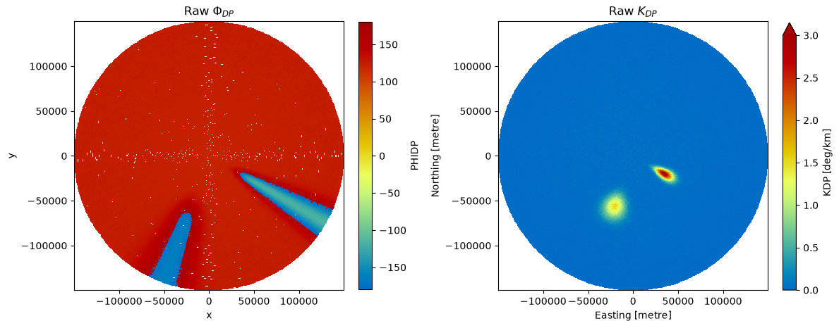
Let’s have a look how the synthetic \(\Phi_{DP}\) and \(K_{DP}\) look like
fig, (ax1, ax2) = plt.subplots(1, 2, figsize=(12, 5))
phi_raw.wrl.vis.plot(ax=ax1)
ax1.set_title("Raw $\Phi_{DP}$")
kdp_raw.wrl.vis.plot(ax=ax2, vmin=0, vmax=3)
ax2.set_title("Raw $K_{DP}$")
fig.tight_layout()
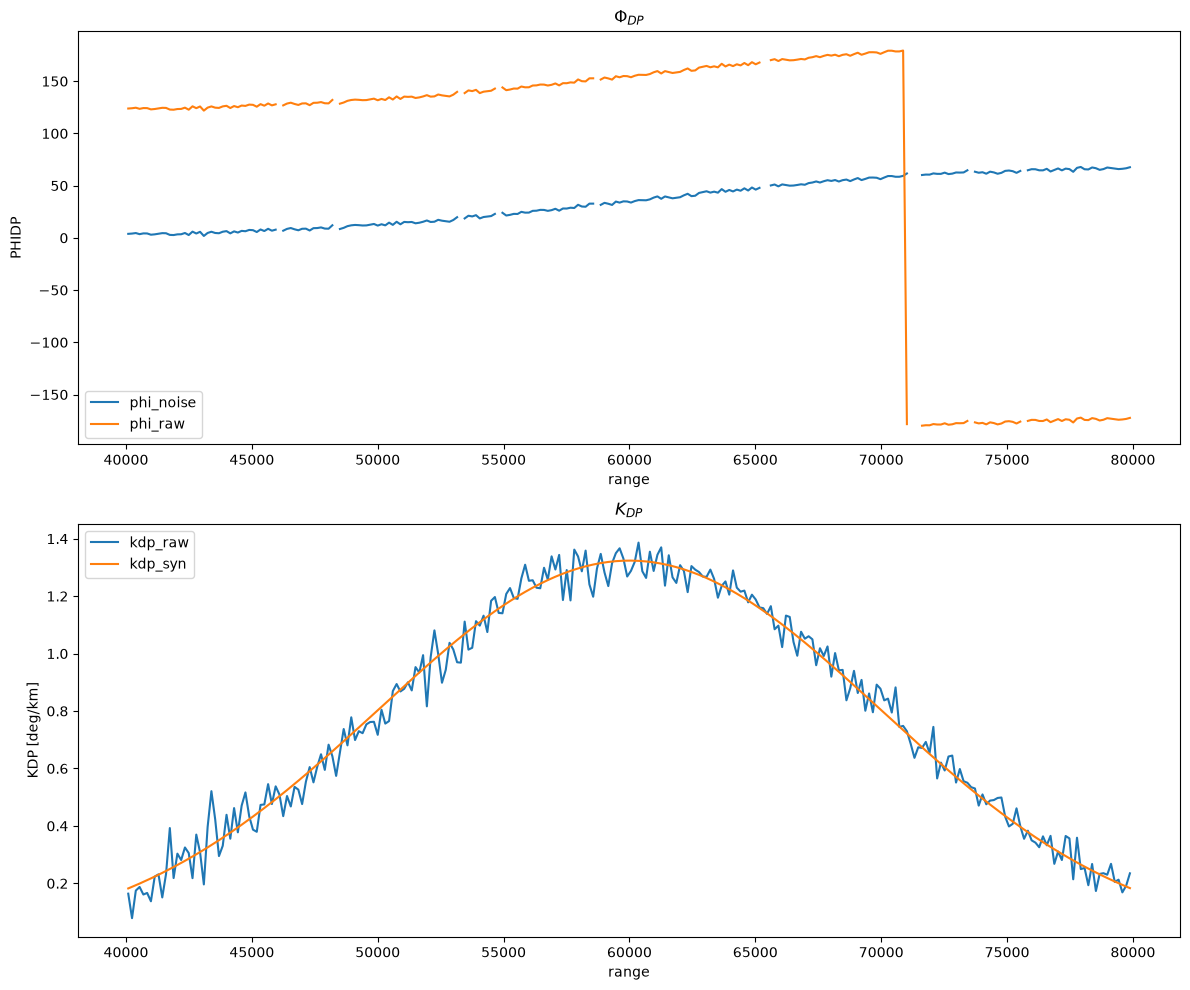
fig, (ax1, ax2) = plt.subplots(2, 1, figsize=(12, 10))
az = 196.0
r = slice(40e3, 80e3)

phi_noise.sel(azimuth=az, range=r).plot.line(ax=ax1, label="phi_noise")
phi_raw.sel(azimuth=az, range=r).plot.line(ax=ax1, label="phi_raw")
ax1.set_title("$\Phi_{DP}$")
ax1.legend(loc="lower left")
kdp_raw.sel(azimuth=az, range=r).plot.line(ax=ax2, label="kdp_raw")
kdp_syn.sel(azimuth=az, range=r).plot.line(ax=ax2, label="kdp_syn")
ax2.set_title("$K_{DP}$")
ax2.legend(loc="upper left")
fig.tight_layout()
Unfold Phase#
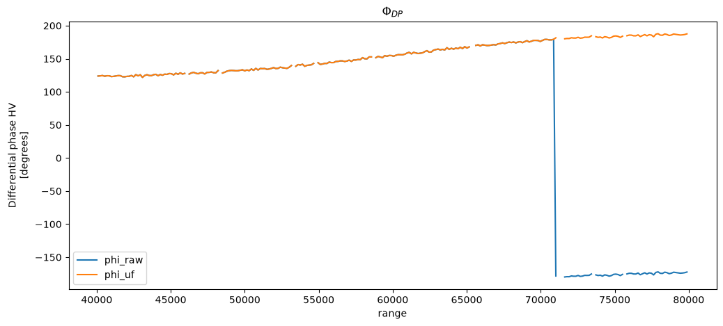
If your radar suffers from phase folding, eg. the phase wraps at 180° and continues to increase from -180 onwards, you would need to proeprly unfold the phase before any subsequent processing. Here we show the unfolding algorith presented in [Vulpiani et al., 2012].
We calculate a first guess \(K_{DP}\) from our \(\Phi_{DP}\) (kdp_from_phidp) and merge both together into one xarray.Dataset.
kdp_der = phi_raw.copy(deep=True).wrl.dp.kdp_from_phidp(winlen=5, method="finite_difference_vulpiani", skipna=False)
ds = xr.merge([phi_raw, kdp_der])
print(ds)
<xarray.Dataset> Size: 23MB
Dimensions:     (azimuth: 360, range: 1000)
Coordinates: (12/14)
  * azimuth     (azimuth) float64 3kB 0.0 1.0 2.0 3.0 ... 357.0 358.0 359.0
    elevation   (azimuth) float64 3kB 1.5 1.5 1.5 1.5 1.5 ... 1.5 1.5 1.5 1.5
  * range       (range) float64 8kB 0.0 150.2 300.3 ... 1.498e+05 1.5e+05
    x           (azimuth, range) float64 3MB 0.0 9.191e-15 ... -2.615e+03
    y           (azimuth, range) float64 3MB 0.0 150.1 ... 1.497e+05 1.498e+05
    z           (azimuth, range) float64 3MB 100.0 103.9 ... 5.341e+03 5.348e+03
    ...          ...
    bins        (azimuth, range) float64 3MB 0.0 150.2 ... 1.498e+05 1.5e+05
    sweep_mode  <U20 80B 'azimuth_surveillance'
    latitude    int64 8B 7
    longitude   int64 8B 50
    altitude    int64 8B 100
    crs_wkt     int64 8B 0
Data variables:
    PHIDP       (azimuth, range) float64 3MB 121.2 119.4 119.5 ... 125.9 125.1
    KDP         (azimuth, range) float64 3MB 0.0 0.8709 -0.06475 ... 0.09325 0.0
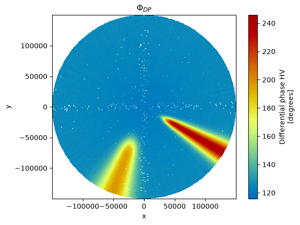
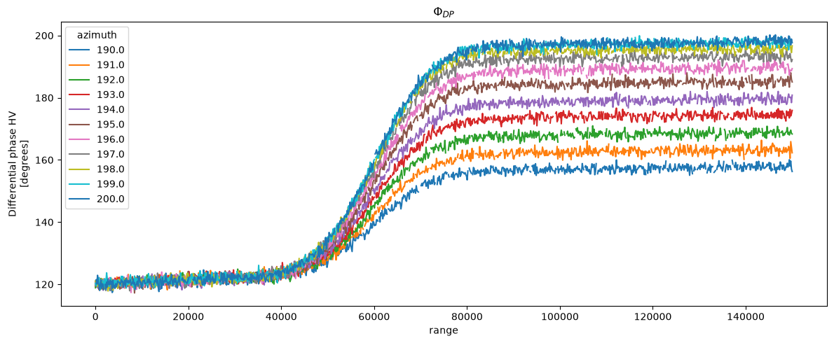
Then we apply the unfolding algorithm (unfold_phi_vulpiani). We additionally check over- and undercorrections.
phi_uf = ds.wrl.dp.unfold_phi_vulpiani(winlen=5, phidp="PHIDP", kdp="KDP")
phi_uf = xr.where(phi_uf >= 500, phi_uf - 360, phi_uf)
phi_uf = xr.where(phi_uf <= -150, phi_uf + 360, phi_uf)

plt.figure()
phi_uf.wrl.vis.plot()
plt.gca().set_title("$\Phi_{DP}$")
fig.tight_layout()
plt.figure(figsize=(12, 5))
phi_uf.sel(azimuth=slice(190., 200.)).plot.line(hue="azimuth")
plt.gca().set_title("$\Phi_{DP}$")
plt.tight_layout()
plt.figure(figsize=(12, 5))
phi_raw.sel(azimuth=az, range=r).plot.line(label="phi_raw")
phi_uf.sel(azimuth=az, range=r).plot.line(label="phi_uf")
plt.gca().set_title("$\Phi_{DP}$")
plt.legend(loc="lower left")
fig.tight_layout()
Derive \(K_{DP}\) from \(\Phi_{DP}\)#
Simple derivation#
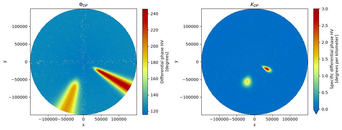
\(\omega radlib\) implements an optimized derivate algorithm which can be shaped for polar phase measurements in kdp_from_phidp.
Using the defaults the derivation algorithm uses low-noise Lanczos Differentiators [Diekema et al., 2012].
winlen should be set to a value where
kdp_der2 = phi_uf.copy(deep=True).wrl.dp.kdp_from_phidp(winlen=47,)
fig, (ax1, ax2) = plt.subplots(1, 2, figsize=(12, 5))
phi_uf.wrl.vis.plot(ax=ax1)
ax1.set_title("$\Phi_{DP}$")
kdp_der2.wrl.vis.plot(ax=ax2, vmin=0, vmax=3)
ax2.set_title("$K_{DP}$")
fig.tight_layout()
Vulpiani Algorithm#
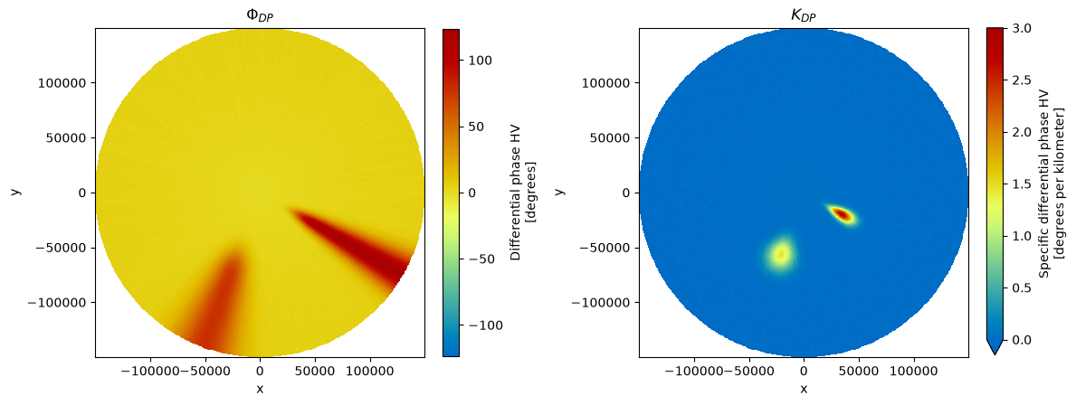
Again in [Vulpiani et al., 2012] a full algorithm for derivation of \(K_{DP}\) from raw \(\Phi_{DP}\) as well as a preprocessed \(\Phi_{DP}\) is described (phidp_kdp_vulpiani).
phi_der, kdp_der3 = phi_uf.copy(deep=True).wrl.dp.phidp_kdp_vulpiani(winlen=47)
fig, (ax1, ax2) = plt.subplots(1, 2, figsize=(12, 5))
phi_der.wrl.vis.plot(ax=ax1)
ax1.set_title("$\Phi_{DP}$")
kdp_der3.wrl.vis.plot(ax=ax2, vmin=0, vmax=3)
ax2.set_title("$K_{DP}$")
fig.tight_layout()
Comparison#
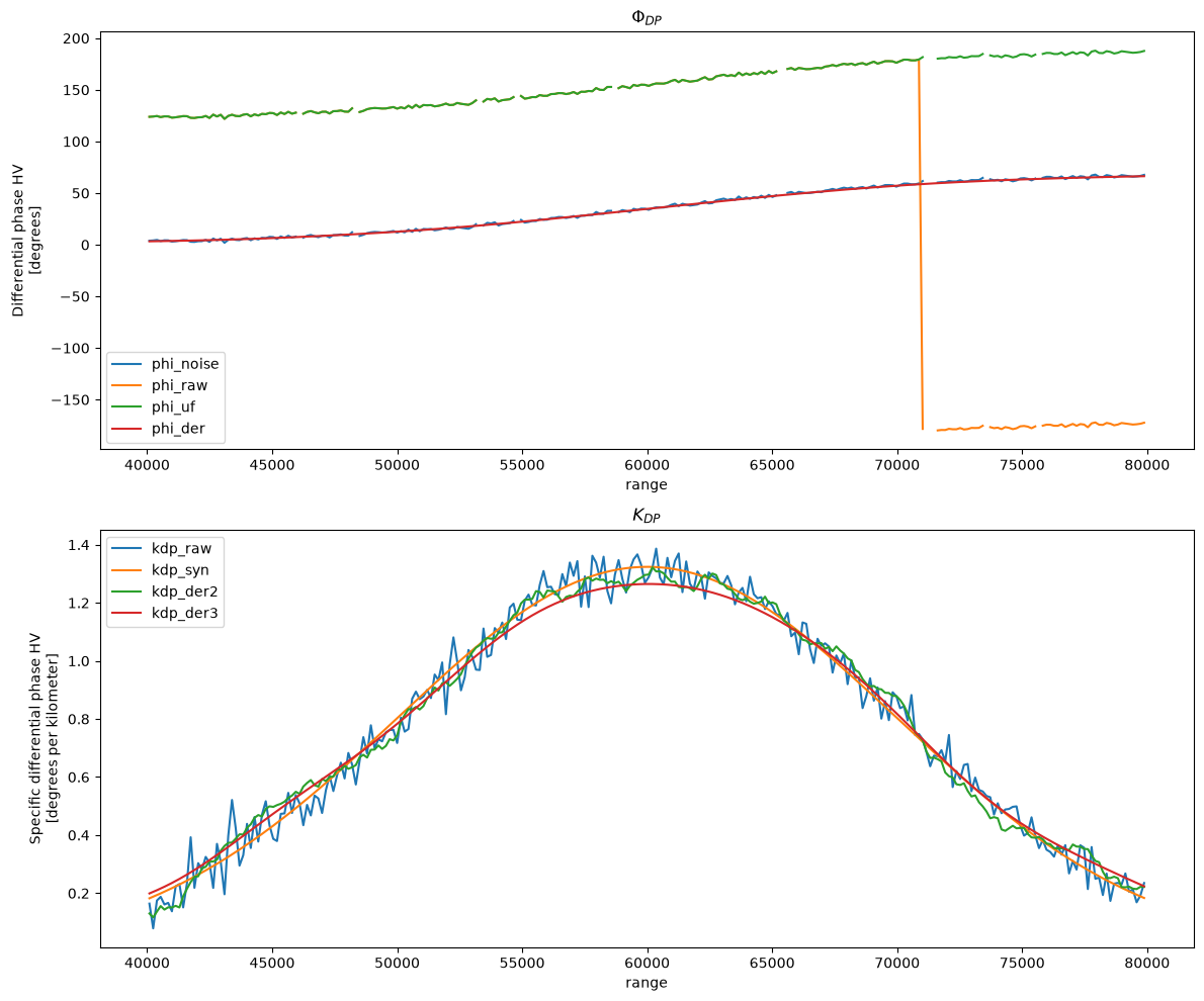
Let’s have a look at the different evolutions of \(\Phi_{DP}\) and \(K_{DP}\).
fig, (ax1, ax2) = plt.subplots(2, 1, figsize=(12, 10))

phi_noise.sel(azimuth=az, range=r).plot.line(ax=ax1, label="phi_noise")
phi_raw.sel(azimuth=az, range=r).plot.line(ax=ax1, label="phi_raw")
phi_uf.sel(azimuth=az, range=r).plot.line(ax=ax1, label="phi_uf")
phi_der.sel(azimuth=az, range=r).plot.line(ax=ax1, label="phi_der")
ax1.set_title("$\Phi_{DP}$")
ax1.legend(loc="lower left")

kdp_raw.sel(azimuth=az, range=r).plot.line(ax=ax2, label="kdp_raw")
kdp_syn.sel(azimuth=az, range=r).plot.line(ax=ax2, label="kdp_syn")
kdp_der2.sel(azimuth=az, range=r).plot.line(ax=ax2, label="kdp_der2")
kdp_der3.sel(azimuth=az, range=r).plot.line(ax=ax2, label="kdp_der3")
ax2.set_title("$K_{DP}$")
ax2.legend(loc="upper left")
fig.tight_layout()