Heuristic clutter detection based on distribution properties (“histo cut”)#
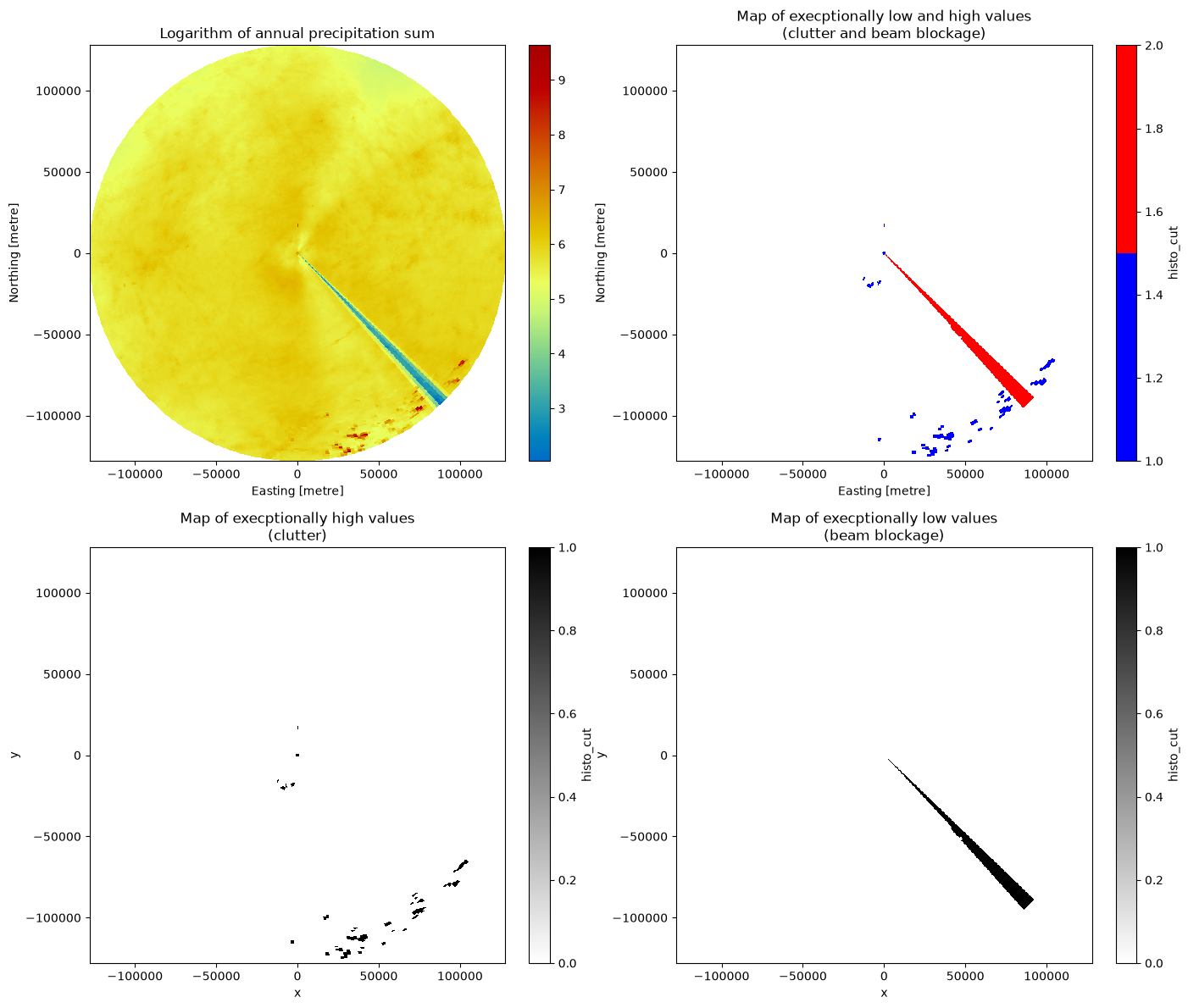
Detects areas with anomalously low or high average reflectivity or precipitation. It is recommended to use long term average or sums (months to year).
import warnings

import matplotlib.pyplot as plt
import numpy as np
import wradlib as wrl
import wradlib_data
import xarray as xr

warnings.filterwarnings("ignore")
/home/docs/checkouts/readthedocs.org/user_builds/wradlib/conda/latest/lib/python3.13/site-packages/tqdm/auto.py:21: TqdmWarning: IProgress not found. Please update jupyter and ipywidgets. See https://ipywidgets.readthedocs.io/en/stable/user_install.html
  from .autonotebook import tqdm as notebook_tqdm
Load rainfall data#
This imports annual rainfall data from DWD radar Feldberg.
filename = wradlib_data.DATASETS.fetch("misc/annual_rainfall_fbg.gz")
yearsum = np.loadtxt(filename)
site = (47.875, 8.004, 1489.6)
r = np.arange(0, 128000, 1000) + 500
az = np.arange(0, 360, 1) + 0.5

fbg = wrl.georef.create_xarray_dataarray(yearsum, r=r, phi=az, site=site).wrl.georef.georeference()
display(fbg)
Downloading file 'misc/annual_rainfall_fbg.gz' from 'https://github.com/wradlib/wradlib-data/raw/main/data/misc/annual_rainfall_fbg.gz' to '/home/docs/.cache/wradlib-data'.
<xarray.DataArray (azimuth: 360, range: 128)> Size: 369kB
array([[672.15, 332.51, 289.34, ..., 219.97, 207.52, 195.32],
       [684.01, 332.6 , 286.18, ..., 208.3 , 202.8 , 199.21],
       [696.95, 329.28, 290.22, ..., 208.42, 207.71, 211.72],
       ...,
       [718.53, 338.63, 297.95, ..., 216.14, 211.72, 205.65],
       [693.46, 344.42, 296.3 , ..., 230.68, 217.27, 202.93],
       [697.33, 331.63, 294.01, ..., 240.7 , 224.42, 200.69]],
      shape=(360, 128))
Coordinates: (12/14)
  * azimuth     (azimuth) float64 3kB 0.5 1.5 2.5 3.5 ... 357.5 358.5 359.5
    elevation   (azimuth) float64 3kB 0.0 0.0 0.0 0.0 0.0 ... 0.0 0.0 0.0 0.0
  * range       (range) float64 1kB 500.0 1.5e+03 ... 1.265e+05 1.275e+05
    x           (azimuth, range) float64 369kB 4.363 13.09 ... -1.112e+03
    y           (azimuth, range) float64 369kB 499.9 1.5e+03 ... 1.275e+05
    z           (azimuth, range) float64 369kB 1.49e+03 1.49e+03 ... 2.445e+03
    ...          ...
    bins        (azimuth, range) float64 369kB 500.0 1.5e+03 ... 1.275e+05
    longitude   float64 8B 47.88
    latitude    float64 8B 8.004
    altitude    float64 8B 1.49e+03
    sweep_mode  <U20 80B 'azimuth_surveillance'
crs_wkt int64 8B 0Apply histo-cut filter#
Depending on your data and climate you can parameterize the upper and lower frequency percentage with the kwargs upper_frequency/lower_frequency. For European ODIM_H5 data these values have been found to be in the order of 0.05 [Overeem et al., 2023]. The current default is 0.01 for both values.
clutter = fbg.wrl.classify.histo_cut()
display(clutter)
<xarray.DataArray 'histo_cut' (azimuth: 360, range: 128)> Size: 46kB
array([[1, 0, 0, ..., 0, 0, 0],
       [1, 0, 0, ..., 0, 0, 0],
       [1, 0, 0, ..., 0, 0, 0],
       ...,
       [1, 0, 0, ..., 0, 0, 0],
       [1, 0, 0, ..., 0, 0, 0],
       [1, 0, 0, ..., 0, 0, 0]], shape=(360, 128), dtype=uint8)
Coordinates: (12/14)
  * azimuth     (azimuth) float64 3kB 0.5 1.5 2.5 3.5 ... 357.5 358.5 359.5
    elevation   (azimuth) float64 3kB 0.0 0.0 0.0 0.0 0.0 ... 0.0 0.0 0.0 0.0
  * range       (range) float64 1kB 500.0 1.5e+03 ... 1.265e+05 1.275e+05
    x           (azimuth, range) float64 369kB 4.363 13.09 ... -1.112e+03
    y           (azimuth, range) float64 369kB 499.9 1.5e+03 ... 1.275e+05
    z           (azimuth, range) float64 369kB 1.49e+03 1.49e+03 ... 2.445e+03
    ...          ...
    bins        (azimuth, range) float64 369kB 500.0 1.5e+03 ... 1.275e+05
    longitude   float64 8B 47.88
    latitude    float64 8B 8.004
    altitude    float64 8B 1.49e+03
    sweep_mode  <U20 80B 'azimuth_surveillance'
crs_wkt int64 8B 0Plot results#
fig = plt.figure(figsize=(14, 12))
ax1 = fig.add_subplot(221)
pm = np.log(fbg).wrl.vis.plot(ax=ax1)
ax1.set_title("Logarithm of annual precipitation sum")
ax2 = fig.add_subplot(222)
cmap2 = plt.get_cmap("bwr", 2)
pm = clutter.where(clutter > 0).wrl.vis.plot(ax=ax2, cmap=cmap2)
ax2.set_title("Map of execptionally low and high values\n(clutter and beam blockage)")
ax3 = fig.add_subplot(223)
pm = xr.where(clutter == 1, 1, 0).wrl.vis.plot(ax=ax3, cmap="binary")
ax3.set_title("Map of execptionally high values\n(clutter)")
ax4 = fig.add_subplot(224)
pm = xr.where(clutter == 2, 1, 0).wrl.vis.plot(ax=ax4, cmap="binary")
ax4.set_title("Map of execptionally low values\n(beam blockage)")
fig.tight_layout()