import datetime as dt
import urllib
import warnings

import matplotlib as mpl
import matplotlib.pyplot as plt
import numpy as np
import wradlib as wrl
import wradlib_data
import xarray as xr
import xradar as xd
from IPython.display import display

warnings.filterwarnings("ignore")
/home/docs/checkouts/readthedocs.org/user_builds/wradlib/conda/latest/lib/python3.13/site-packages/tqdm/auto.py:21: TqdmWarning: IProgress not found. Please update jupyter and ipywidgets. See https://ipywidgets.readthedocs.io/en/stable/user_install.html
  from .autonotebook import tqdm as notebook_tqdm
2D Hydrometeor Classification#
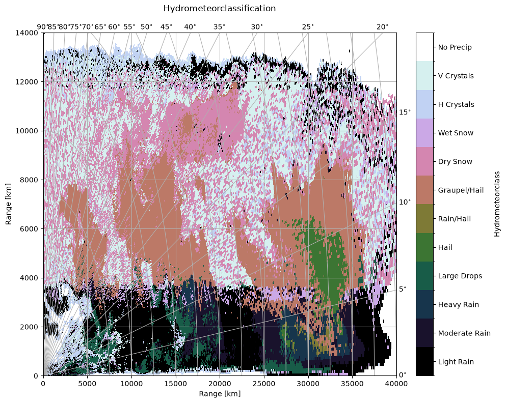
The hydrometeorclassification code is based on the paper by [Zrnic et al., 2001] utilizing 2D trapezoidal membership functions based on the paper by [Straka et al., 2000] adapted by [Evaristo et al., 2013] for X-Band.
Precipitation Types#
pr_types = wrl.classify.pr_types
for k, v in pr_types.items():
    print(str(k) + " - ".join(v))
0LR - Light Rain
1MR - Moderate Rain
2HR - Heavy Rain
3LD - Large Drops
4HL - Hail
5RH - Rain/Hail
6GH - Graupel/Hail
7DS - Dry Snow
8WS - Wet Snow
9HC - H Crystals
10VC - V Crystals
11NP - No Precip
Membership Functions#
filename = wradlib_data.DATASETS.fetch("misc/msf_xband_v1.nc")
msf = xr.open_dataset(filename)
display(msf)
Downloading file 'misc/msf_xband_v1.nc' from 'https://github.com/wradlib/wradlib-data/raw/main/data/misc/msf_xband_v1.nc' to '/home/docs/.cache/wradlib-data'.
<xarray.Dataset> Size: 97kB
Dimensions:  (hmc: 11, idp: 55, trapezoid: 4)
Coordinates:
  * hmc      (hmc) <U2 88B 'LR' 'MR' 'HR' 'LD' 'HL' ... 'GH' 'DS' 'WS' 'HC' 'VC'
  * idp      (idp) float64 440B -10.0 -8.0 -6.0 -4.0 ... 92.0 94.0 96.0 98.0
Dimensions without coordinates: trapezoid
Data variables:
    ZH       (hmc, idp, trapezoid) float64 19kB ...
    ZDR      (hmc, idp, trapezoid) float64 19kB ...
    RHO      (hmc, idp, trapezoid) float64 19kB ...
    KDP      (hmc, idp, trapezoid) float64 19kB ...
    TEMP     (hmc, idp, trapezoid) float64 19kB ...
Attributes:
    version:      1
    title:        2D Membershipfunctions Hydrometeorclassification for XBand
    institution:  Institute of Geosciences, Meteorology Section, University o...
    history:      created by Raquel Evaristo, adapted to netCDF by Kai Mühlbauer
comment: created with wradlibUse Sounding Data#
Retrieve Sounding Data#
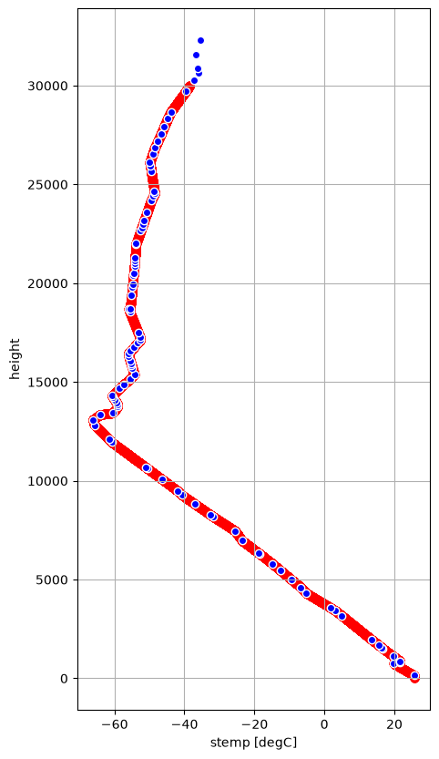
To get the temperature as additional discriminator we use radiosonde data from the University of Wyoming.
The function wradlib.io.misc.get_radiosonde tries to find the next next available radiosonde measurement on the given date.
rs_time = dt.datetime(2014, 6, 10, 12, 0)

try:
    rs_data, rs_meta = wrl.io.get_radiosonde(10410, rs_time)
except (urllib.error.HTTPError, urllib.error.URLError):
    dataf = wradlib_data.DATASETS.fetch("misc/radiosonde_10410_20140610_1200.h5")
    rs_data, _ = wrl.io.from_hdf5(dataf)
    metaf = wradlib_data.DATASETS.fetch("misc/radiosonde_10410_20140610_1200.json")
    with open(metaf, "r") as infile:
        import json

        rs_meta = json.load(infile)
rs_meta
Downloading file 'misc/radiosonde_10410_20140610_1200.h5' from 'https://github.com/wradlib/wradlib-data/raw/main/data/misc/radiosonde_10410_20140610_1200.h5' to '/home/docs/.cache/wradlib-data'.
Downloading file 'misc/radiosonde_10410_20140610_1200.json' from 'https://github.com/wradlib/wradlib-data/raw/main/data/misc/radiosonde_10410_20140610_1200.json' to '/home/docs/.cache/wradlib-data'.
{'Station identifier': 'EDZE',
 'Station number': 10410,
 'Station latitude': 51.4,
 'Station longitude': 6.96,
 'Station elevation': 153.0,
 'Showalter index': 1.65,
 'Lifted index': -5.84,
 'LIFT computed using virtual temperature': -6.23,
 'SWEAT index': 89.02,
 'K index': 23.7,
 'Cross totals index': 17.3,
 'Vertical totals index': 31.3,
 'Totals totals index': 48.6,
 'Convective Available Potential Energy': 1536.47,
 'CAPE using virtual temperature': 1637.41,
 'Convective Inhibition': -140.01,
 'CINS using virtual temperature': -80.22,
 'Equilibrum Level': 202.61,
 'Equilibrum Level using virtual temperature': 202.55,
 'Level of Free Convection': 735.93,
 'LFCT using virtual temperature': 772.57,
 'Bulk Richardson Number': 57.19,
 'Bulk Richardson Number using CAPV': 60.94,
 'Temp [K] of the Lifted Condensation Level': 288.2,
 'Pres [hPa] of the Lifted Condensation Level': 882.1,
 'Mean mixed layer potential temperature': 298.74,
 'Mean mixed layer mixing ratio': 12.41,
 '1000 hPa to 500 hPa thickness': 5657.0,
 'Precipitable water [mm] for entire sounding': 28.11,
 'quantity': {'PRES': 'hPa',
  'HGHT': 'm',
  'TEMP': 'C',
  'DWPT': 'C',
  'FRPT': 'C',
  'RELH': '%',
  'RELI': '%',
  'MIXR': 'g/kg',
  'DRCT': 'deg',
  'SKNT': 'knot',
  'THTA': 'K',
  'THTE': 'K',
  'THTV': 'K'}}
Extract Temperature and Height#
stemp = rs_data["TEMP"]
sheight = rs_data["HGHT"]
# remove nans
idx = np.isfinite(stemp)
stemp = stemp[idx]
sheight = sheight[idx]
Create DataArray#
stemp_da = xr.DataArray(
    data=stemp,
    dims=["height"],
    coords=dict(
        height=(["height"], sheight),
    ),
    attrs=dict(
        description="Temperature.",
        units="degC",
    ),
)
display(stemp_da)
<xarray.DataArray (height: 97)> Size: 776B
array([ 25.6,  19.8,  21.6,  21.6,  21.6,  19.7,  16.7,  16.4,  15.6,
        13.4,   5. ,   3.2,   1.8,  -5.3,  -6.7,  -9.3, -12.5, -14.9,
       -18.5, -18.9, -23.5, -25.5, -31.9, -32.7, -37. , -40.7, -41.9,
       -46.5, -50.5, -51.1, -60.7, -61.5, -65.7, -66.1, -64.1, -60.5,
       -59.1, -59.1, -59.4, -59.9, -60.4, -60.7, -58.5, -57.4, -55.5,
       -54.3, -54.9, -55.1, -55.3, -55.5, -55.9, -56.1, -55.4, -54.4,
       -53.4, -52.5, -52.7, -53.2, -55.6, -55.9, -55.5, -55.1, -54.9,
       -54.8, -54.6, -54.5, -54.3, -54.2, -54.2, -54.1, -53.9, -53.8,
       -52.5, -52.2, -51.8, -51.5, -50.7, -49.5, -48.9, -48.5, -48.6,
       -49.5, -49.7, -49.9, -49.1, -48.5, -47.6, -46.7, -45.8, -44.8,
       -43.9, -39.5, -37.3, -35.9, -36.1, -36.7, -35.5])
Coordinates:
  * height   (height) float64 776B 153.0 745.0 828.0 ... 3.155e+04 3.228e+04
Attributes:
    description:  Temperature.
units: degCInterpolate to higher resolution#
hmax = 30000.0
ht = np.arange(0.0, hmax)
itemp_da = stemp_da.interp({"height": ht})
display(itemp_da)
<xarray.DataArray (height: 30000)> Size: 240kB
array([         nan,          nan,          nan, ..., -38.47842779,
       -38.47440585, -38.47038391], shape=(30000,))
Coordinates:
  * height   (height) float64 240kB 0.0 1.0 2.0 3.0 ... 3e+04 3e+04 3e+04 3e+04
Attributes:
    description:  Temperature.
units: degCFix Temperature below first measurement#
itemp_da = itemp_da.bfill(dim="height")
Plot Temperature Profile#
fig = plt.figure(figsize=(5, 10))
ax = fig.add_subplot(111)
itemp_da.plot(y="height", ax=ax, marker="o", zorder=0, c="r")
stemp_da.to_dataset(name="stemp").plot.scatter(
    x="stemp", y="height", ax=ax, marker="o", c="b", zorder=1
)
ax.grid(True)
Prepare Radar Data#
Load Radar Data#
# read the radar volume scan
filename = "hdf5/2014-06-09--185000.rhi.mvol"
filename = wradlib_data.DATASETS.fetch(filename)
Downloading file 'hdf5/2014-06-09--185000.rhi.mvol' from 'https://github.com/wradlib/wradlib-data/raw/main/data/hdf5/2014-06-09--185000.rhi.mvol' to '/home/docs/.cache/wradlib-data'.
Extract data for georeferencing#
swp = xr.open_dataset(
    filename, engine="gamic", group="sweep_0", chunks={}
)
swp = xd.util.remove_duplicate_rays(swp)
swp = xd.util.reindex_angle(
    swp, start_angle=0, stop_angle=90, angle_res=0.2, direction=1
)
display(swp)
<xarray.Dataset> Size: 14MB
Dimensions:            (range: 667, elevation: 450)
Coordinates:
  * range              (range) float32 3kB 37.5 112.5 ... 4.991e+04 4.999e+04
  * elevation          (elevation) float64 4kB 0.1 0.3 0.5 ... 89.5 89.7 89.9
    azimuth            (elevation) float64 4kB dask.array<chunksize=(450,), meta=np.ndarray>
    time               (elevation) datetime64[ns] 4kB dask.array<chunksize=(450,), meta=np.ndarray>
    longitude          float64 8B ...
    latitude           float64 8B ...
    altitude           float64 8B ...
Data variables: (12/18)
    KDP                (elevation, range) float32 1MB dask.array<chunksize=(450, 667), meta=np.ndarray>
    PHIDP              (elevation, range) float32 1MB dask.array<chunksize=(450, 667), meta=np.ndarray>
    DBZH               (elevation, range) float32 1MB dask.array<chunksize=(450, 667), meta=np.ndarray>
    DBZV               (elevation, range) float32 1MB dask.array<chunksize=(450, 667), meta=np.ndarray>
    RHOHV              (elevation, range) float32 1MB dask.array<chunksize=(450, 667), meta=np.ndarray>
    DBTH               (elevation, range) float32 1MB dask.array<chunksize=(450, 667), meta=np.ndarray>
    ...                 ...
    sweep_mode         <U3 12B ...
    sweep_number       int64 8B ...
    prt_mode           <U7 28B ...
    follow_mode        <U7 28B ...
    sweep_fixed_angle  float64 8B ...
    nyquist_velocity   object 8B ...
Attributes:
    source:       gamic
pulse_width: 0Get Heights of Radar Bins#
swp = swp.wrl.georef.georeference()
display(swp)
<xarray.Dataset> Size: 28MB
Dimensions:            (range: 667, elevation: 450)
Coordinates: (12/14)
  * range              (range) float32 3kB 37.5 112.5 ... 4.991e+04 4.999e+04
    x                  (elevation, range) float64 2MB -26.52 -79.55 ... -61.32
    y                  (elevation, range) float64 2MB -26.52 -79.55 ... -61.34
    z                  (elevation, range) float64 2MB 99.57 99.7 ... 5.009e+04
    gr                 (elevation, range) float64 2MB 18.39 93.39 ... 67.62
    rays               (elevation, range) float64 2MB 0.1 0.1 0.1 ... 89.9 89.9
    ...                 ...
    azimuth            (elevation) float64 4kB dask.array<chunksize=(450,), meta=np.ndarray>
    time               (elevation) datetime64[ns] 4kB dask.array<chunksize=(450,), meta=np.ndarray>
    longitude          float64 8B ...
    latitude           float64 8B ...
    altitude           float64 8B ...
    crs_wkt            int64 8B 0
Data variables: (12/18)
    KDP                (elevation, range) float32 1MB dask.array<chunksize=(450, 667), meta=np.ndarray>
    PHIDP              (elevation, range) float32 1MB dask.array<chunksize=(450, 667), meta=np.ndarray>
    DBZH               (elevation, range) float32 1MB dask.array<chunksize=(450, 667), meta=np.ndarray>
    DBZV               (elevation, range) float32 1MB dask.array<chunksize=(450, 667), meta=np.ndarray>
    RHOHV              (elevation, range) float32 1MB dask.array<chunksize=(450, 667), meta=np.ndarray>
    DBTH               (elevation, range) float32 1MB dask.array<chunksize=(450, 667), meta=np.ndarray>
    ...                 ...
    sweep_mode         <U3 12B ...
    sweep_number       int64 8B ...
    prt_mode           <U7 28B ...
    follow_mode        <U7 28B ...
    sweep_fixed_angle  float64 8B ...
    nyquist_velocity   object 8B ...
Attributes:
    source:       gamic
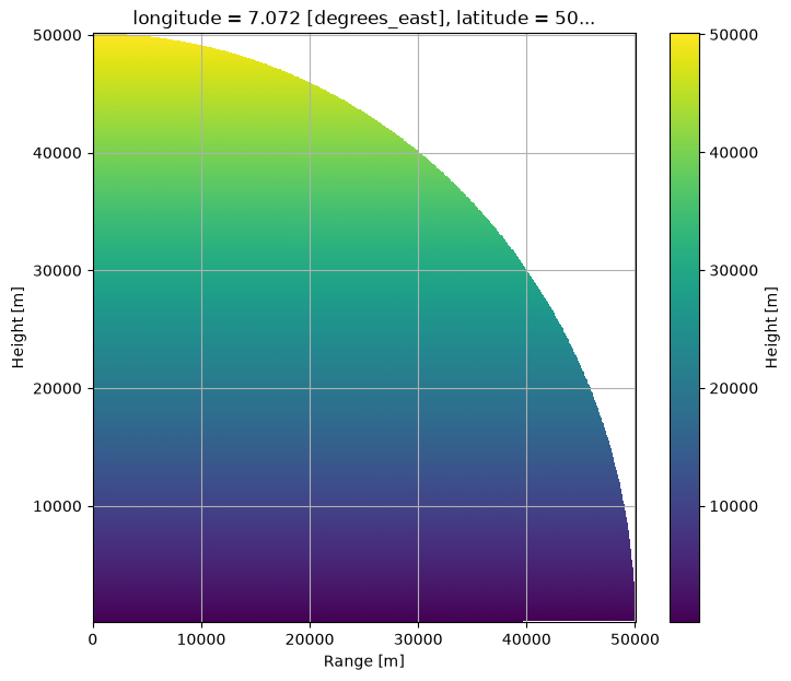
pulse_width: 0Plot RHI of Heights#
fig = plt.figure(figsize=(8, 7))
ax = fig.add_subplot(111)
cmap = mpl.cm.viridis
swp.z.plot(x="gr", y="z", ax=ax, cbar_kwargs=dict(label="Height [m]"))
ax.set_xlabel("Range [m]")
ax.set_ylabel("Height [m]")
ax.grid(True)
plt.show()
Get Index into High Res Height Array#
def merge_radar_profile(rds, cds):
    cds = cds.interp({"height": rds.z}, method="linear")
    rds = rds.assign({"TEMP": cds})
    return rds
hmc_ds = swp.pipe(merge_radar_profile, itemp_da)
display(hmc_ds)
<xarray.Dataset> Size: 32MB
Dimensions:            (range: 667, elevation: 450)
Coordinates: (12/15)
  * range              (range) float32 3kB 37.5 112.5 ... 4.991e+04 4.999e+04
    x                  (elevation, range) float64 2MB -26.52 -79.55 ... -61.32
    y                  (elevation, range) float64 2MB -26.52 -79.55 ... -61.34
    z                  (elevation, range) float64 2MB 99.57 99.7 ... 5.009e+04
    gr                 (elevation, range) float64 2MB 18.39 93.39 ... 67.62
    rays               (elevation, range) float64 2MB 0.1 0.1 0.1 ... 89.9 89.9
    ...                 ...
    azimuth            (elevation) float64 4kB dask.array<chunksize=(450,), meta=np.ndarray>
    time               (elevation) datetime64[ns] 4kB dask.array<chunksize=(450,), meta=np.ndarray>
    longitude          float64 8B ...
    latitude           float64 8B ...
    altitude           float64 8B ...
    crs_wkt            int64 8B 0
Data variables: (12/19)
    KDP                (elevation, range) float32 1MB dask.array<chunksize=(450, 667), meta=np.ndarray>
    PHIDP              (elevation, range) float32 1MB dask.array<chunksize=(450, 667), meta=np.ndarray>
    DBZH               (elevation, range) float32 1MB dask.array<chunksize=(450, 667), meta=np.ndarray>
    DBZV               (elevation, range) float32 1MB dask.array<chunksize=(450, 667), meta=np.ndarray>
    RHOHV              (elevation, range) float32 1MB dask.array<chunksize=(450, 667), meta=np.ndarray>
    DBTH               (elevation, range) float32 1MB dask.array<chunksize=(450, 667), meta=np.ndarray>
    ...                 ...
    sweep_number       int64 8B ...
    prt_mode           <U7 28B ...
    follow_mode        <U7 28B ...
    sweep_fixed_angle  float64 8B ...
    nyquist_velocity   object 8B ...
    TEMP               (elevation, range) float64 2MB 25.6 25.6 25.6 ... nan nan
Attributes:
    source:       gamic
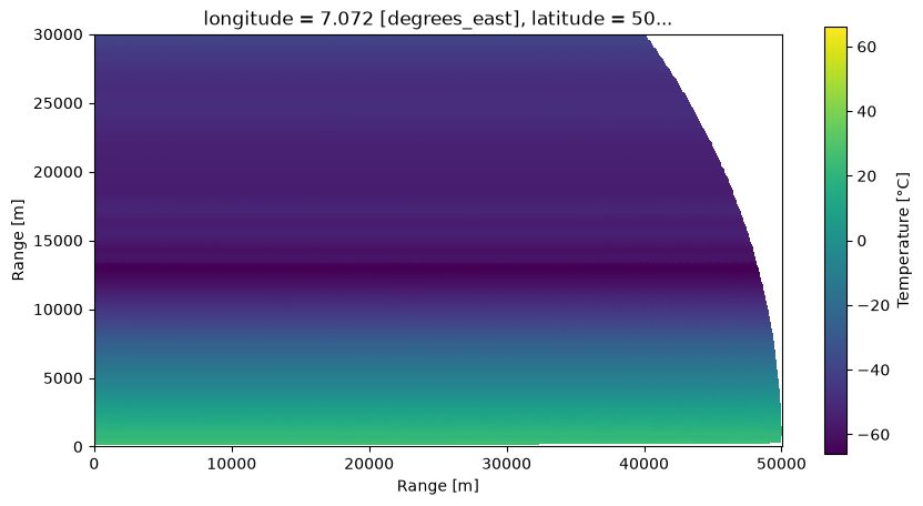
pulse_width: 0fig = plt.figure(figsize=(10, 5))
ax = fig.add_subplot(111)
hmc_ds.TEMP.plot(
x="gr",
y="z",
cmap=cmap,
ax=ax,
add_colorbar=True,
cbar_kwargs=dict(label="Temperature [°C]"),
)
ax.set_xlabel("Range [m]")
ax.set_ylabel("Range [m]")
ax.set_aspect("equal")
ax.set_ylim(0, 30000)
plt.show()
HMC Workflow#
Setup Independent Observable \(Z_H\)#
Retrieve membership function values based on independent observable
%%time
msf_val = msf.wrl.classify.msf_index_indep(swp.DBZH)
display(msf_val)
<xarray.DataArray 'msf_index_indep' (hmc: 11, obs: 5, elevation: 450,
                                     range: 667, trapezoid: 4)> Size: 264MB
dask.array<transpose, shape=(11, 5, 450, 667, 4), dtype=int32, chunksize=(11, 5, 450, 667, 4), chunktype=numpy.ndarray>
Coordinates: (12/16)
  * hmc        (hmc) <U2 88B 'LR' 'MR' 'HR' 'LD' 'HL' ... 'DS' 'WS' 'HC' 'VC'
  * obs        (obs) object 40B 'ZH' 'ZDR' 'RHO' 'KDP' 'TEMP'
  * elevation  (elevation) float64 4kB 0.1 0.3 0.5 0.7 ... 89.3 89.5 89.7 89.9
    azimuth    (elevation) float64 4kB dask.array<chunksize=(450,), meta=np.ndarray>
    time       (elevation) datetime64[ns] 4kB dask.array<chunksize=(450,), meta=np.ndarray>
  * range      (range) float32 3kB 37.5 112.5 187.5 ... 4.991e+04 4.999e+04
    ...         ...
    rays       (elevation, range) float64 2MB 0.1 0.1 0.1 0.1 ... 89.9 89.9 89.9
    bins       (elevation, range) float32 1MB 37.5 112.5 ... 4.991e+04 4.999e+04
    longitude  float64 8B ...
    latitude   float64 8B ...
    altitude   float64 8B ...
    crs_wkt    int64 8B 0
Dimensions without coordinates: trapezoid
Attributes:
    version:      1
    title:        2D Membershipfunctions Hydrometeorclassification for XBand
    institution:  Institute of Geosciences, Meteorology Section, University o...
    history:      created by Raquel Evaristo, adapted to netCDF by Kai Mühlbauer
comment: created with wradlibCPU times: user 18 ms, sys: 0 ns, total: 18 ms
Wall time: 18.1 ms
Fuzzyfication#
%%time
fu = msf_val.wrl.classify.fuzzyfi(
    hmc_ds, dict(ZH="DBZH", ZDR="ZDR", RHO="RHOHV", KDP="KDP", TEMP="TEMP")
)
CPU times: user 6.96 ms, sys: 713 μs, total: 7.67 ms
Wall time: 9.14 ms
Probability#
# weights dataset
w = xr.Dataset(dict(ZH=2.0, ZDR=1.0, RHO=1.0, KDP=1.0, TEMP=1.0))
display(w)
<xarray.Dataset> Size: 40B
Dimensions:  ()
Data variables:
    ZH       float64 8B 2.0
    ZDR      float64 8B 1.0
    RHO      float64 8B 1.0
    KDP      float64 8B 1.0
TEMP float64 8B 1.0%%time
prob = fu.wrl.classify.probability(w).compute()
display(prob)
<xarray.DataArray (hmc: 11, elevation: 450, range: 667)> Size: 26MB
array([[[0.16666667, 0.5       , 0.5       , ..., 0.        ,
         0.        , 0.        ],
        [0.        , 0.5       , 0.66666667, ..., 0.        ,
         0.        , 0.        ],
        [0.        , 0.5       , 0.5       , ..., 0.        ,
         0.        , 0.        ],
        ...,
        [0.16666667, 0.66666667, 0.5       , ..., 0.        ,
         0.        , 0.        ],
        [0.16666667, 0.66666667, 0.5       , ..., 0.        ,
         0.        , 0.        ],
        [0.16666667, 0.66666667, 0.5       , ..., 0.        ,
         0.        , 0.        ]],

       [[0.        , 0.        , 0.        , ..., 0.        ,
         0.        , 0.        ],
        [0.        , 0.        , 0.        , ..., 0.        ,
         0.        , 0.        ],
        [0.        , 0.        , 0.        , ..., 0.        ,
         0.        , 0.        ],
...
        [0.29812113, 0.33333333, 0.33333333, ..., 0.        ,
         0.        , 0.        ],
        [0.31296539, 0.33333333, 0.33333333, ..., 0.        ,
         0.        , 0.        ],
        [0.32917684, 0.33333333, 0.33333333, ..., 0.        ,
         0.        , 0.        ]],

       [[0.29480082, 0.33333333, 0.33333333, ..., 0.        ,
         0.        , 0.        ],
        [0.25280711, 0.33333333, 0.33333333, ..., 0.        ,
         0.        , 0.        ],
        [0.25808055, 0.33333333, 0.33333333, ..., 0.        ,
         0.        , 0.        ],
        ...,
        [0.29812113, 0.33333333, 0.33333333, ..., 0.        ,
         0.        , 0.        ],
        [0.31296539, 0.33333333, 0.33333333, ..., 0.        ,
         0.        , 0.        ],
        [0.32917684, 0.33333333, 0.33333333, ..., 0.        ,
         0.        , 0.        ]]], shape=(11, 450, 667))
Coordinates: (12/16)
  * hmc        (hmc) <U2 88B 'LR' 'MR' 'HR' 'LD' 'HL' ... 'DS' 'WS' 'HC' 'VC'
  * elevation  (elevation) float64 4kB 0.1 0.3 0.5 0.7 ... 89.3 89.5 89.7 89.9
    azimuth    (elevation) float64 4kB 225.0 225.0 225.0 ... 225.0 225.0 225.0
    time       (elevation) datetime64[ns] 4kB 2014-06-09T18:50:01 ... 2014-06...
  * range      (range) float32 3kB 37.5 112.5 187.5 ... 4.991e+04 4.999e+04
    x          (elevation, range) float64 2MB -26.52 -79.55 ... -61.23 -61.32
    ...         ...
    bins       (elevation, range) float32 1MB 37.5 112.5 ... 4.991e+04 4.999e+04
    height     (elevation, range) float64 2MB 99.57 99.7 ... 5.001e+04 5.009e+04
    longitude  float64 8B 7.072
    latitude   float64 8B 50.73
    altitude   float64 8B 99.5
    crs_wkt    int64 8B 0
Attributes:
    version:      1
    title:        2D Membershipfunctions Hydrometeorclassification for XBand
    institution:  Institute of Geosciences, Meteorology Section, University o...
    history:      created by Raquel Evaristo, adapted to netCDF by Kai Mühlbauer
comment: created with wradlibCPU times: user 600 ms, sys: 229 ms, total: 829 ms
Wall time: 760 ms
# prob = prob.compute()
Classification#
cl_res = prob.wrl.classify.classify(threshold=0.0)
display(cl_res)
<xarray.DataArray (hmc: 12, elevation: 450, range: 667)> Size: 29MB
array([[[0.16666667, 0.5       , 0.5       , ..., 0.        ,
         0.        , 0.        ],
        [0.        , 0.5       , 0.66666667, ..., 0.        ,
         0.        , 0.        ],
        [0.        , 0.5       , 0.5       , ..., 0.        ,
         0.        , 0.        ],
        ...,
        [0.16666667, 0.66666667, 0.5       , ..., 0.        ,
         0.        , 0.        ],
        [0.16666667, 0.66666667, 0.5       , ..., 0.        ,
         0.        , 0.        ],
        [0.16666667, 0.66666667, 0.5       , ..., 0.        ,
         0.        , 0.        ]],

       [[0.        , 0.        , 0.        , ..., 0.        ,
         0.        , 0.        ],
        [0.        , 0.        , 0.        , ..., 0.        ,
         0.        , 0.        ],
        [0.        , 0.        , 0.        , ..., 0.        ,
         0.        , 0.        ],
...
        [0.29812113, 0.33333333, 0.33333333, ..., 0.        ,
         0.        , 0.        ],
        [0.31296539, 0.33333333, 0.33333333, ..., 0.        ,
         0.        , 0.        ],
        [0.32917684, 0.33333333, 0.33333333, ..., 0.        ,
         0.        , 0.        ]],

       [[0.        , 0.        , 0.        , ..., 1.        ,
         1.        , 1.        ],
        [0.        , 0.        , 0.        , ..., 1.        ,
         1.        , 1.        ],
        [0.        , 0.        , 0.        , ..., 1.        ,
         1.        , 1.        ],
        ...,
        [0.        , 0.        , 0.        , ..., 1.        ,
         1.        , 1.        ],
        [0.        , 0.        , 0.        , ..., 1.        ,
         1.        , 1.        ],
        [0.        , 0.        , 0.        , ..., 1.        ,
         1.        , 1.        ]]], shape=(12, 450, 667))
Coordinates: (12/16)
  * hmc        (hmc) <U2 96B 'LR' 'MR' 'HR' 'LD' 'HL' ... 'WS' 'HC' 'VC' 'NP'
  * elevation  (elevation) float64 4kB 0.1 0.3 0.5 0.7 ... 89.3 89.5 89.7 89.9
    azimuth    (elevation) float64 4kB 225.0 225.0 225.0 ... 225.0 225.0 225.0
    time       (elevation) datetime64[ns] 4kB 2014-06-09T18:50:01 ... 2014-06...
  * range      (range) float32 3kB 37.5 112.5 187.5 ... 4.991e+04 4.999e+04
    x          (elevation, range) float64 2MB -26.52 -79.55 ... -61.23 -61.32
    ...         ...
    bins       (elevation, range) float32 1MB 37.5 112.5 ... 4.991e+04 4.999e+04
    height     (elevation, range) float64 2MB 99.57 99.7 ... 5.001e+04 5.009e+04
    longitude  float64 8B 7.072
    latitude   float64 8B 50.73
    altitude   float64 8B 99.5
    crs_wkt    int64 8B 0
Attributes:
    version:      1
    title:        2D Membershipfunctions Hydrometeorclassification for XBand
    institution:  Institute of Geosciences, Meteorology Section, University o...
    history:      created by Raquel Evaristo, adapted to netCDF by Kai Mühlbauer
comment: created with wradlibCompute#
%%time
cl_res = cl_res.compute()
cl_res = cl_res.assign_coords(sweep_mode="rhi")
display(cl_res)
<xarray.DataArray (hmc: 12, elevation: 450, range: 667)> Size: 29MB
array([[[0.16666667, 0.5       , 0.5       , ..., 0.        ,
         0.        , 0.        ],
        [0.        , 0.5       , 0.66666667, ..., 0.        ,
         0.        , 0.        ],
        [0.        , 0.5       , 0.5       , ..., 0.        ,
         0.        , 0.        ],
        ...,
        [0.16666667, 0.66666667, 0.5       , ..., 0.        ,
         0.        , 0.        ],
        [0.16666667, 0.66666667, 0.5       , ..., 0.        ,
         0.        , 0.        ],
        [0.16666667, 0.66666667, 0.5       , ..., 0.        ,
         0.        , 0.        ]],

       [[0.        , 0.        , 0.        , ..., 0.        ,
         0.        , 0.        ],
        [0.        , 0.        , 0.        , ..., 0.        ,
         0.        , 0.        ],
        [0.        , 0.        , 0.        , ..., 0.        ,
         0.        , 0.        ],
...
        [0.29812113, 0.33333333, 0.33333333, ..., 0.        ,
         0.        , 0.        ],
        [0.31296539, 0.33333333, 0.33333333, ..., 0.        ,
         0.        , 0.        ],
        [0.32917684, 0.33333333, 0.33333333, ..., 0.        ,
         0.        , 0.        ]],

       [[0.        , 0.        , 0.        , ..., 1.        ,
         1.        , 1.        ],
        [0.        , 0.        , 0.        , ..., 1.        ,
         1.        , 1.        ],
        [0.        , 0.        , 0.        , ..., 1.        ,
         1.        , 1.        ],
        ...,
        [0.        , 0.        , 0.        , ..., 1.        ,
         1.        , 1.        ],
        [0.        , 0.        , 0.        , ..., 1.        ,
         1.        , 1.        ],
        [0.        , 0.        , 0.        , ..., 1.        ,
         1.        , 1.        ]]], shape=(12, 450, 667))
Coordinates: (12/17)
* hmc (hmc) <U2 96B 'LR' 'MR' 'HR' 'LD' 'HL' ... 'WS' 'HC' 'VC' 'NP'
* elevation (elevation) float64 4kB 0.1 0.3 0.5 0.7 ... 89.3 89.5 89.7 89.9
azimuth (elevation) float64 4kB 225.0 225.0 225.0 ... 225.0 225.0 225.0
time (elevation) datetime64[ns] 4kB 2014-06-09T18:50:01 ... 2014-0...
* range (range) float32 3kB 37.5 112.5 187.5 ... 4.991e+04 4.999e+04
x (elevation, range) float64 2MB -26.52 -79.55 ... -61.23 -61.32
... ...
height (elevation, range) float64 2MB 99.57 99.7 ... 5.009e+04
longitude float64 8B 7.072
latitude float64 8B 50.73
altitude float64 8B 99.5
crs_wkt int64 8B 0
sweep_mode <U3 12B 'rhi'
Attributes:
version: 1
title: 2D Membershipfunctions Hydrometeorclassification for XBand
institution: Institute of Geosciences, Meteorology Section, University o...
history: created by Raquel Evaristo, adapted to netCDF by Kai Mühlbauer
comment: created with wradlibCPU times: user 22.7 ms, sys: 2.1 ms, total: 24.8 ms
Wall time: 23.7 ms
HMC Results#
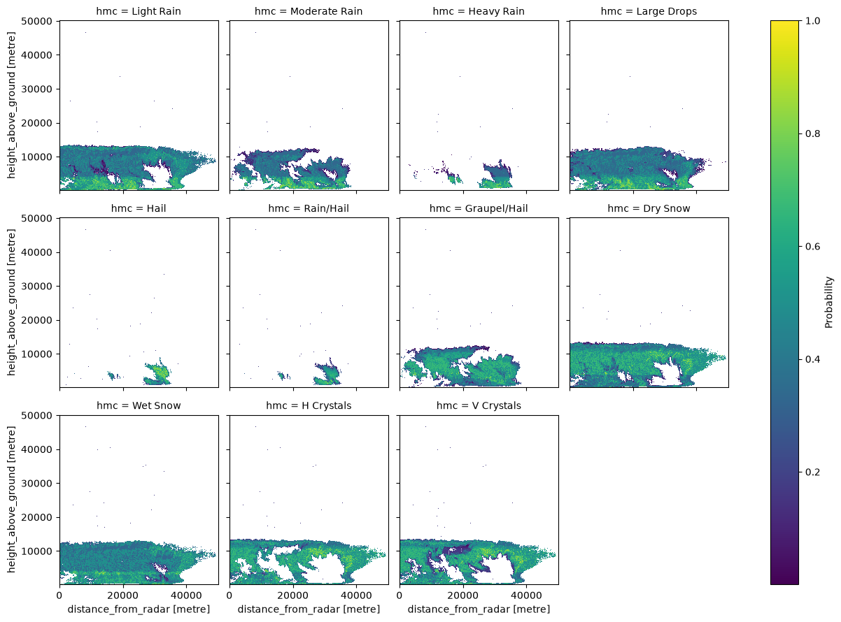
Plot Probability of HMC Types#
prob = prob.assign_coords(hmc=np.array(list(pr_types.values())).T[1][:11])
prob = prob.where(prob > 0)
prob.plot(x="gr", y="z", col="hmc", col_wrap=4, cbar_kwargs=dict(label="Probability"))
<xarray.plot.facetgrid.FacetGrid at 0x7a2a7498d010>
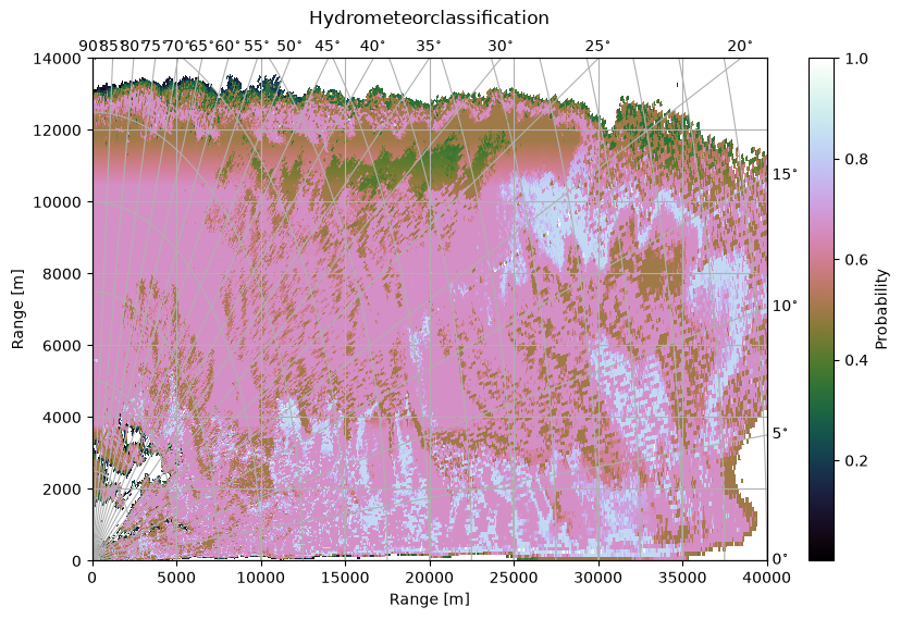
Plot maximum probability#
fig = plt.figure(figsize=(10, 6))
cmap = "cubehelix"
kwargs=dict(cbar_kwargs=dict(label="Probability"))
print(kwargs)
im = cl_res.max("hmc").wrl.vis.plot(
    ax=111,
    crs={"angular_spacing": 20.0, "radial_spacing": 12.0, "latmin": 2.5},
    cmap=cmap,
    fig=fig,
    **kwargs,
)
cgax = plt.gca()
cgax.set_xlim(0, 40000)
cgax.set_ylim(0, 14000)
t = cgax.set_title("Hydrometeorclassification", y=1.05)

caax = cgax.parasites[0]
caax.set_xlabel("Range [m]")
caax.set_ylabel("Range [m]")
plt.show()
{'cbar_kwargs': {'label': 'Probability'}}
Plot classification result#
bounds = np.arange(-0.5, prob.shape[0] + 0.6, 1)
ticks = np.arange(0, prob.shape[0] + 1)
cmap = plt.get_cmap("cubehelix", len(ticks))
norm = mpl.colors.BoundaryNorm(bounds, cmap.N)
hydro = cl_res.argmax("hmc")
hydro.attrs = dict(long_name="Hydrometeorclassification")
hydro = hydro.assign_coords(sweep_mode="rhi")
fig = plt.figure(figsize=(10, 8))
im = hydro.wrl.vis.plot(
    ax=111,
    crs={"angular_spacing": 20.0, "radial_spacing": 12.0, "latmin": 2.5},
    norm=norm,
    cmap=cmap,
    fig=fig,
    add_colorbar=False,
)
cgax = plt.gca()
caax = cgax.parasites[0]
paax = cgax.parasites[1]

cbar = plt.colorbar(im, ticks=ticks, ax=cgax, fraction=0.046, norm=norm, pad=0.05)
cbar.set_label("Hydrometeorclass")
caax.set_xlabel("Range [km]")
caax.set_ylabel("Range [km]")
labels = [pr_types[i][1] for i, _ in enumerate(pr_types)]
labels = cbar.ax.set_yticklabels(labels)
t = cgax.set_title("Hydrometeorclassification", y=1.05)
cgax.set_xlim(0, 40000)
cgax.set_ylim(0, 14000)
plt.tight_layout()