Path-Integrated Attenuation#
This notebook demonstrates the core attenuation correction capabilities of wradlib.atten module, including the unconstrained [Hitschfeld et al., 1954] approach dating back to 1954. It compares the different approaches to constrain the gate-by-gate retrieval of path-integrated attenuation.
Rainfall-induced attenuation is a major source of underestimation for radar-based precipitation estimation at C-band and X-band. Unconstrained forward gate-by-gate correction is known to be inherently unstable and thus not suited for unsupervised quality control procedures. Ideally, reference measurements (e.g. from microwave links) should be used to constrain gate-by-gate procedures. However, such attenuation references are usually not available. \(\omega radlib\) provides a pragmatic approach to constrain gate-by-gate correction procedures, inspired by the work of [Kraemer et al., 2008]. It turned out that these procedures can effectively reduce the error introduced by attenuation, and, at the same time, minimize instability issues [Jacobi et al., 2016].
import numpy as np
import matplotlib.pyplot as plt
import wradlib as wrl
import wradlib_data
import warnings
import xarray as xr
import cmweather

warnings.filterwarnings("ignore")
try:
    get_ipython().run_line_magic("matplotlib inline")
except:
    plt.ion()
/home/docs/checkouts/readthedocs.org/user_builds/wradlib/conda/latest/lib/python3.13/site-packages/tqdm/auto.py:21: TqdmWarning: IProgress not found. Please update jupyter and ipywidgets. See https://ipywidgets.readthedocs.io/en/stable/user_install.html
  from .autonotebook import tqdm as notebook_tqdm
Read a polar data set#
Let’s have a look at the situation in South-West Germany on June 2nd, 2008, at 16:55 UTC, as observed by the DWD C-band radar on mount Feldberg.
fname = wradlib_data.DATASETS.fetch("dx/raa00-dx_10908-0806021655-fbg---bin.gz")
data, attrs = wrl.io.read_dx(fname)
da = wrl.georef.create_xarray_dataarray(data).wrl.georef.georeference()
display(da)
Downloading file 'dx/raa00-dx_10908-0806021655-fbg---bin.gz' from 'https://github.com/wradlib/wradlib-data/raw/main/data/dx/raa00-dx_10908-0806021655-fbg---bin.gz' to '/home/docs/.cache/wradlib-data'.
<xarray.DataArray (azimuth: 360, range: 128)> Size: 369kB
array([[-10. , -18.5, -26.5, ..., -32.5, -32.5, -32.5],
       [-19. , -19.5, -14. , ..., -32.5, -32.5, -32.5],
       [-15. , -21. , -32.5, ..., -32.5, -32.5, -32.5],
       ...,
       [ -0.5, -15.5, -32.5, ..., -32.5, -32.5, -32.5],
       [  1.5, -18.5, -19. , ..., -32.5, -32.5, -32.5],
       [ -2.5, -20.5, -32.5, ..., -32.5, -32.5, -32.5]], shape=(360, 128))
Coordinates: (12/14)
  * azimuth     (azimuth) float64 3kB 0.5 1.5 2.5 3.5 ... 357.5 358.5 359.5
    elevation   (azimuth) float64 3kB 0.0 0.0 0.0 0.0 0.0 ... 0.0 0.0 0.0 0.0
  * range       (range) float64 1kB 0.5 1.5 2.5 3.5 ... 124.5 125.5 126.5 127.5
    x           (azimuth, range) float64 369kB 0.004363 0.01309 ... -1.113
    y           (azimuth, range) float64 369kB 0.5 1.5 2.5 ... 125.5 126.5 127.5
    z           (azimuth, range) float64 369kB 1.49e-08 1.322e-07 ... 0.0009558
    ...          ...
    bins        (azimuth, range) float64 369kB 0.5 1.5 2.5 ... 125.5 126.5 127.5
    longitude   float64 8B 0.0
    latitude    float64 8B 0.0
    altitude    float64 8B 0.0
    sweep_mode  <U20 80B 'azimuth_surveillance'
crs_wkt int64 8B 0Overview Plot#
# plot raw reflectivity
pm = da.wrl.vis.plot(vmin=0, vmax=60)
sel = da.isel(azimuth=53)
plt.gca().plot(
    [sel.x[0], sel.x[-1]], [sel.y[0], sel.y[-1]], "r-", lw=2
)
plt.title("Raw Reflectivity (dBZ)")
Text(0.5, 1.0, 'Raw Reflectivity (dBZ)')
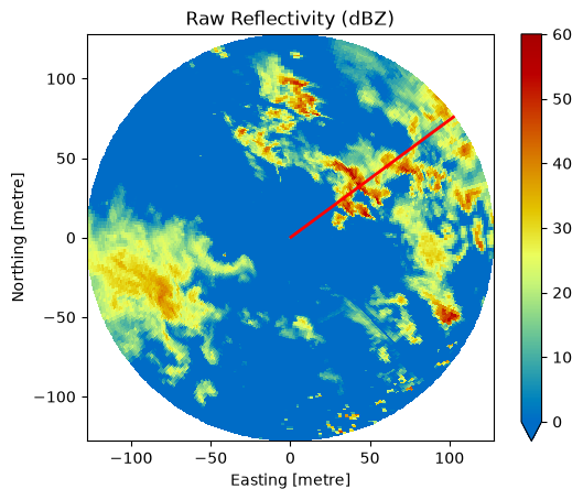
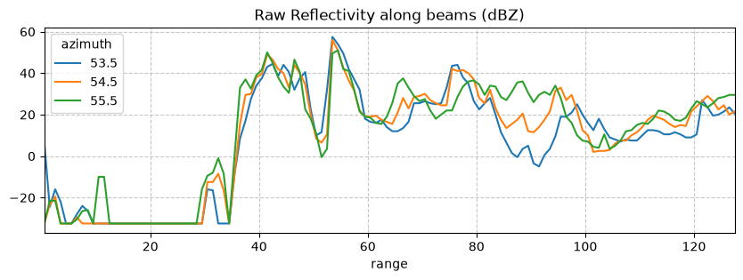
We see a set of convective cells with high rainfall intensity in the NE-sector of the Feldberg radar. Let us examine the reflectivity profile along three beams which are at azimuths 53-55 degree (as marked by the white line in the PPI above).
fig, ax = plt.subplots(1, 1, figsize=(10, 3))
sel = da.sel(azimuth=slice(53, 56))
sel.plot.line(ax=ax, hue="azimuth")
ax.grid(True, which='both', linestyle='--', alpha=0.7)
ax.set_xlim(float(sel.range.min()), float(sel.range.max()))
ax.set_title("Raw Reflectivity along beams (dBZ)")
Text(0.5, 1.0, 'Raw Reflectivity along beams (dBZ)')
1. Hitschfeld and Bordan#
First, we examine the behaviour of the “classical” unconstrained forward correction which is typically referred to [Hitschfeld et al., 1954], although Hitschfeld and Bordan themselves rejected this approach. The Path Integrated Attenuation (PIA) according to this approach can be obtained as follows:
pia_hibo = da.wrl.atten.correct_attenuation_hb(
    coefficients=dict(a=8.0e-5, b=0.731, gate_length=1.0), mode="warn", thrs=59.0
)
corrected signal over threshold (59.0)
In the coefficients dictionary, we can pass the power law parameters of the A(Z) relation as well as the gate length (in km). If we pass “warn” as the mode argument, we will obtain a warning log in case the corrected reflectivity exceeds the value of argument thrs (dBZ).
Plotting the result below the reflectivity profile, we obtain the following figure.
fig, (ax1, ax2) = plt.subplots(2, 1, figsize=(10, 6))
sel = da.sel(azimuth=slice(53, 56))
sel.plot.line(ax=ax1, hue="azimuth")
ax1.grid(True, which='both', linestyle='--', alpha=0.7)
ax1.set_xlim(float(sel.range.min()), float(sel.range.max()))
ax1.set_title("Raw Reflectivity along beams (dBZ)")
sel2 = pia_hibo.sel(azimuth=slice(53, 56))
sel2.plot.line(ax=ax2, hue="azimuth")
ax2.grid(True, which='both', linestyle='--', alpha=0.7)
ax2.set_xlim(float(sel.range.min()), float(sel.range.max()))
ax2.set_ylim(0, 30)
ax2.set_title("PIA according to Hitschfeld and Bordan")
plt.tight_layout()
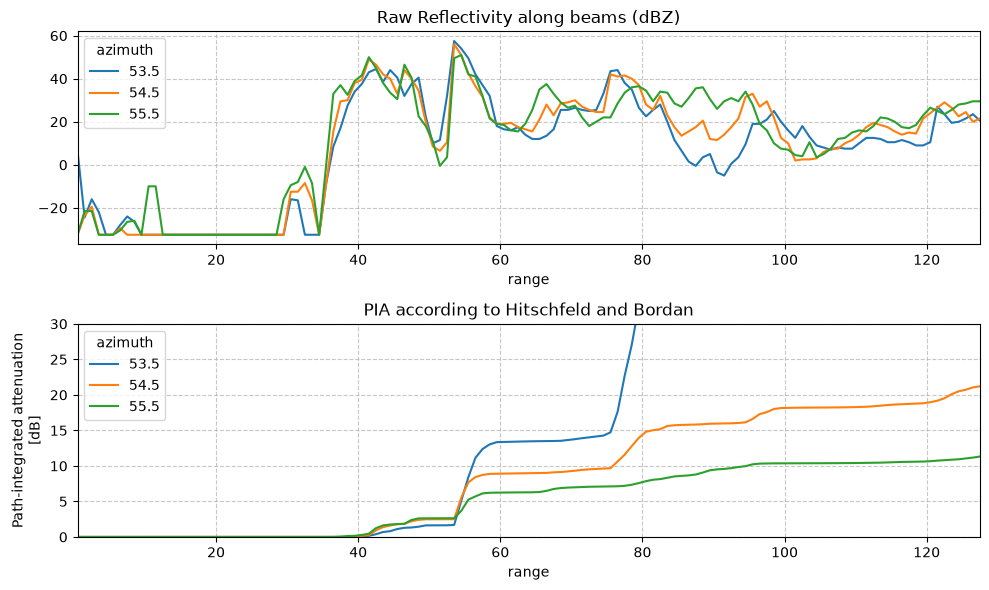
Apparently, slight differences in the reflectivity profile can cause a dramatic change in the behaviour. While at 54.5 and 55.5 degrees, the retrieval of PIA appears to be fairly stable, the profile of PIA for 53.5 degree demonstrates a case of instability.
2. Harrison#
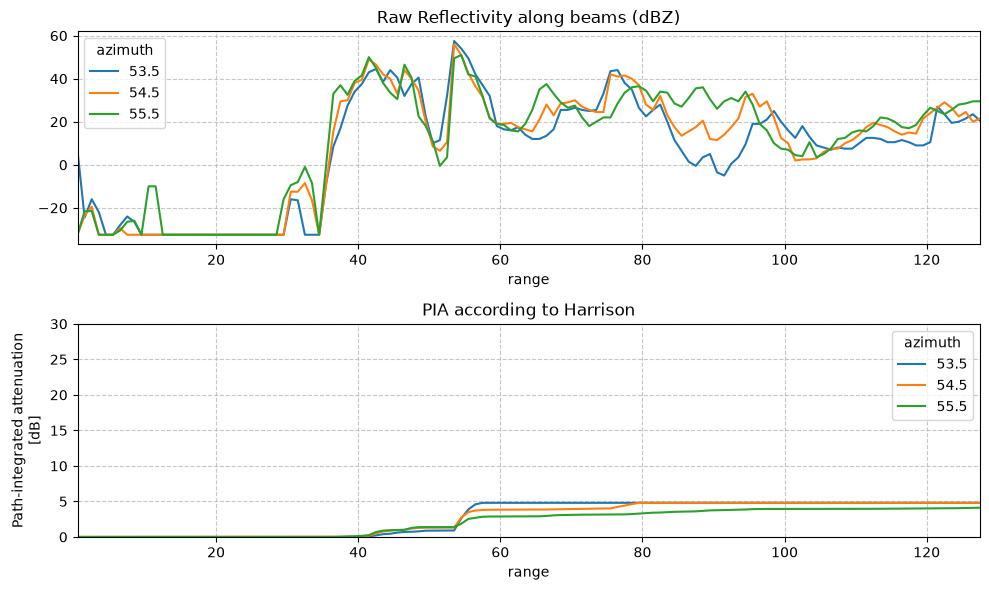
[Harrison et al., 2000] suggested to simply cap PIA in case it would cause a correction of rainfall intensity by more than a factor of two. Depending on the parameters of the Z(R) relationship, that would correpond to PIA values between 4 and 5 dB (4.8 dB if we assume exponent b=1.6).
One way to implement this approach would be the following:
pia_harrison = da.wrl.atten.correct_attenuation_hb(coefficients=dict(a=4.57e-5, b=0.731, gate_length=1.0), mode="warn", thrs=59.0
)
pia_harrison = pia_harrison.clip(max=4.8)
And the results would look like this:
fig, (ax1, ax2) = plt.subplots(2, 1, figsize=(10, 6))
sel = da.sel(azimuth=slice(53, 56))
sel.plot.line(ax=ax1, hue="azimuth")
ax1.grid(True, which='both', linestyle='--', alpha=0.7)
ax1.set_xlim(float(sel.range.min()), float(sel.range.max()))
ax1.set_title("Raw Reflectivity along beams (dBZ)")
sel2 = pia_harrison.sel(azimuth=slice(53, 56))
sel2.plot.line(ax=ax2, hue="azimuth")
ax2.grid(True, which='both', linestyle='--', alpha=0.7)
ax2.set_xlim(float(sel.range.min()), float(sel.range.max()))
ax2.set_ylim(0, 30)
ax2.set_title("PIA according to Harrison")
plt.tight_layout()
3. Kraemer#
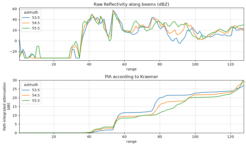
[Kraemer et al., 2008] suggested to iteratively determine the power law parameters of the A(Z). In particular, the power law coefficient is interatively decreased until the attenuation correction does not lead to reflectivity values above a given threshold (Kraemer suggested 59 dBZ). Using \(\omega radlib\), this would be called by using the function correct_attenuation_constrained with a specific constraints argument:
pia_kraemer = da.wrl.atten.correct_attenuation_constrained(
    a_max=1.67e-4,
    a_min=2.33e-5,
    n_a=100,
    b_max=0.7,
    b_min=0.65,
    n_b=6,
    gate_length=1.0,
    constraints=[wrl.atten.constraint_dbz],
    constraint_args=[[59.0]],
)
In brief, this call specifies ranges of the power parameters a and b of the A(Z) relation. Beginning from the maximum values (a_max and b_max), the function searches for values of a and b so that the corrected reflectivity will not exceed the dBZ constraint of 59 dBZ. Compared to the previous results, the corresponding profiles of PIA look like this:
fig, (ax1, ax2) = plt.subplots(2, 1, figsize=(10, 6))
sel = da.sel(azimuth=slice(53, 56))
sel.plot.line(ax=ax1, hue="azimuth")
ax1.grid(True, which='both', linestyle='--', alpha=0.7)
ax1.set_xlim(float(sel.range.min()), float(sel.range.max()))
ax1.set_title("Raw Reflectivity along beams (dBZ)")
sel2 = pia_kraemer.sel(azimuth=slice(53, 56))
sel2.plot.line(ax=ax2, hue="azimuth")
ax2.grid(True, which='both', linestyle='--', alpha=0.7)
ax2.set_xlim(float(sel.range.min()), float(sel.range.max()))
ax2.set_ylim(0, 30)
ax2.set_title("PIA according to Kraemer")
plt.tight_layout()
4. Modified Kraemer#
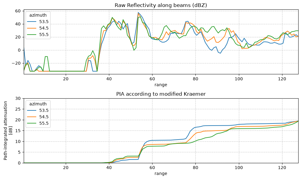
The function correct_attenuation_constrained allows us to pass any kind of constraint function or lists of constraint functions via the argument constraints. The arguments of these functions are passed via a nested list as argument constraint_args. For example, [Jacobi et al., 2016] suggested to constrain both the corrected reflectivity (by a maximum of 59 dBZ) and the resulting path-intgrated attenuation PIA (by a maximum of 20 dB):
pia_mkraemer = da.wrl.atten.correct_attenuation_constrained(
    a_max=1.67e-4,
    a_min=2.33e-5,
    n_a=100,
    b_max=0.7,
    b_min=0.65,
    n_b=6,
    gate_length=1.0,
    constraints=[wrl.atten.constraint_dbz, wrl.atten.constraint_pia],
    constraint_args=[[59.0], [20.0]],
)
fig, (ax1, ax2) = plt.subplots(2, 1, figsize=(10, 6))
sel = da.sel(azimuth=slice(53, 56))
sel.plot.line(ax=ax1, hue="azimuth")
ax1.grid(True, which='both', linestyle='--', alpha=0.7)
ax1.set_xlim(float(sel.range.min()), float(sel.range.max()))
ax1.set_title("Raw Reflectivity along beams (dBZ)")
sel2 = pia_mkraemer.sel(azimuth=slice(53, 56))
sel2.plot.line(ax=ax2, hue="azimuth")
ax2.grid(True, which='both', linestyle='--', alpha=0.7)
ax2.set_xlim(float(sel.range.min()), float(sel.range.max()))
ax2.set_ylim(0, 30)
ax2.set_title("PIA according to modified Kraemer")
plt.tight_layout()
Comparison#
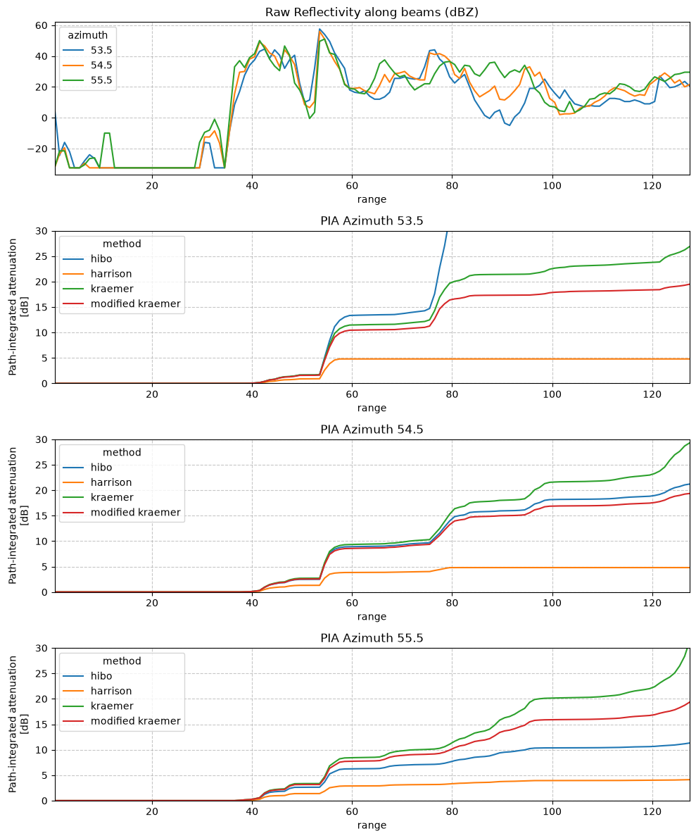
Plotting all of the above methods (Hitschfeld and Bordan, Harrison, Kraemer, Modified Kraemer allows for a better comparison of their behaviour. Please refer to [Jacobi et al., 2016] for an in-depth discussion of this example.
pia_list = [pia_hibo, pia_harrison, pia_kraemer, pia_mkraemer]
pia_all = xr.concat(pia_list, dim="method").assign_coords(method=["hibo", "harrison", "kraemer", "modified kraemer"])
pia_all = pia_all.sel(azimuth=slice(53, 56))

fig, axes = plt.subplots(4, 1, figsize=(10, 12))

sel = da.sel(azimuth=slice(53, 56))
ax1 = axes[0]
sel.plot.line(ax=ax1, hue="azimuth")
ax1.grid(True, which='both', linestyle='--', alpha=0.7)
ax1.set_xlim(float(sel.range.min()), float(sel.range.max()))
ax1.set_title("Raw Reflectivity along beams (dBZ)")

for i, ax in enumerate(axes[1:]):
    pia_plot = pia_all.isel(azimuth=i)
    pia_plot.plot.line(hue="method", ax=ax)
    ax.grid(True, linestyle="--", alpha=0.7)
    ax.set_xlim(float(pia_all.range.min()), float(pia_all.range.max()))
    ax.set_ylim(0, 30)
    ax.set_title(f"PIA Azimuth {pia_plot.azimuth.values}")

plt.tight_layout()