Zonal Statistics - Quickstart#
Zonal statistics can be used to compute e.g. the areal average precipitation over a catchment.
Here, we show a brief example using RADOLAN composite data from the German Weather Service (DWD).
[1]:
import wradlib as wrl
import matplotlib.pyplot as pl
import matplotlib as mpl
import warnings

warnings.filterwarnings("ignore")
try:
    get_ipython().run_line_magic("matplotlib inline")
except:
    pl.ion()
import numpy as np
from osgeo import osr
/home/runner/micromamba-root/envs/wradlib-tests/lib/python3.11/site-packages/tqdm/auto.py:22: TqdmWarning: IProgress not found. Please update jupyter and ipywidgets. See https://ipywidgets.readthedocs.io/en/stable/user_install.html
  from .autonotebook import tqdm as notebook_tqdm
[2]:
from matplotlib.collections import PatchCollection
from matplotlib.colors import from_levels_and_colors
import matplotlib.patches as patches
Preparing the RADOLAN data#
Preparing the radar composite data includes to - read the data, - geoference the data in native RADOLAN projection, - reproject the data to UTM zone 32 projection.
[3]:
# Read and preprocess the RADOLAN data
fpath = "radolan/misc/raa01-sf_10000-1406100050-dwd---bin.gz"
f = wrl.util.get_wradlib_data_file(fpath)
ds = wrl.io.open_radolan_dataset(f)
[4]:
gridres = ds.x.diff("x")[0].values
gridres
[4]:
array(1000.)
[5]:
# This is the native RADOLAN projection
# (polar stereographic projection)
# create radolan projection osr object
if ds.attrs["formatversion"] >= 5:
    proj_stereo = wrl.georef.create_osr("dwd-radolan-wgs84")
else:
    proj_stereo = wrl.georef.create_osr("dwd-radolan-sphere")

# This is our target projection (UTM Zone 32)
proj_utm = osr.SpatialReference()
proj_utm.ImportFromEPSG(32632)

# This is the source projection of the shape data
proj_gk2 = osr.SpatialReference()
proj_gk2.ImportFromEPSG(31466)
[5]:
0
[6]:
# Get RADOLAN grid coordinates - center coordinates
x_rad, y_rad = np.meshgrid(ds.x, ds.y)
grid_xy_radolan = np.stack([x_rad, y_rad], axis=-1)
# Reproject the RADOLAN coordinates
xy = wrl.georef.reproject(
    grid_xy_radolan, projection_source=proj_stereo, projection_target=proj_utm
)
# assign as coordinates
ds = ds.assign_coords(
    {
        "xc": (
            ["y", "x"],
            xy[..., 0],
            dict(long_name="UTM Zone 32 Easting", units="m"),
        ),
        "yc": (
            ["y", "x"],
            xy[..., 1],
            dict(long_name="UTM Zone 32 Northing", units="m"),
        ),
    }
)
Fix shapefile without projection information#
As an example it is shown how to fix a shapefile with missing projection information.
[7]:
from osgeo import ogr, osr, gdal
import os

# Shape Source Projection
proj_gk2 = osr.SpatialReference()
proj_gk2.ImportFromEPSG(31466)

# This is our target projection (UTM Zone 32)
proj_utm = osr.SpatialReference()
proj_utm.ImportFromEPSG(32632)

flist = ["shapefiles/agger/agger_merge.shx", "shapefiles/agger/agger_merge.dbf"]
[wrl.util.get_wradlib_data_file(f) for f in flist]
shpfile = wrl.util.get_wradlib_data_file("shapefiles/agger/agger_merge.shp")
dst_shpfile = shpfile[:-4] + "_gk2.shp"


def transform_shapefile(src, dst, dst_srs, dst_driver="ESRI Shapefile", src_srs=None):
    # remove destination file, if exists
    driver = ogr.GetDriverByName(dst_driver)
    if os.path.exists(dst_shpfile):
        driver.DeleteDataSource(dst_shpfile)

    # create the output layer
    dst_ds = driver.CreateDataSource(dst)
    dst_lyr = dst_ds.CreateLayer("", dst_srs, geom_type=ogr.wkbPolygon)

    # get the input layer
    src_ds = gdal.OpenEx(src)
    src_lyr = src_ds.GetLayer()

    # transform - reproject
    wrl.georef.ogr_reproject_layer(src_lyr, dst_lyr, dst_srs, src_srs=src_srs)

    # unlock files
    dst_ds = None
    src_ds = None


transform_shapefile(shpfile, dst_shpfile, proj_gk2, src_srs=proj_gk2)
Import catchment boundaries from ESRI shapefile#
Create trg VectorSource#
This shows how to load data in a specific projection and project it on the fly to another projection. Here gk2 -> utm32.
[8]:
shpfile = wrl.util.get_wradlib_data_file("shapefiles/agger/agger_merge_gk2.shp")
trg = wrl.io.VectorSource(shpfile, srs=proj_utm, name="trg")
print(f"Found {len(trg)} sub-catchments in shapefile.")
Found 13 sub-catchments in shapefile.
[9]:
# check projection
print(trg.crs)
PROJCS["WGS 84 / UTM zone 32N",
    GEOGCS["WGS 84",
        DATUM["WGS_1984",
            SPHEROID["WGS 84",6378137,298.257223563,
                AUTHORITY["EPSG","7030"]],
            AUTHORITY["EPSG","6326"]],
        PRIMEM["Greenwich",0,
            AUTHORITY["EPSG","8901"]],
        UNIT["degree",0.0174532925199433,
            AUTHORITY["EPSG","9122"]],
        AUTHORITY["EPSG","4326"]],
    PROJECTION["Transverse_Mercator"],
    PARAMETER["latitude_of_origin",0],
    PARAMETER["central_meridian",9],
    PARAMETER["scale_factor",0.9996],
    PARAMETER["false_easting",500000],
    PARAMETER["false_northing",0],
    UNIT["metre",1,
        AUTHORITY["EPSG","9001"]],
    AXIS["Easting",EAST],
    AXIS["Northing",NORTH],
    AUTHORITY["EPSG","32632"]]
Clip subgrid from RADOLAN grid#
This is just to speed up the computation (so we don’t have to deal with the full grid).
[10]:
bbox = trg.extent
buffer = 5000.0
bbox = dict(
    left=bbox[0] - buffer,
    right=bbox[1] + buffer,
    bottom=bbox[2] - buffer,
    top=bbox[3] + buffer,
)
print(bbox)
{'left': 365059.5928799211, 'right': 419830.11388741195, 'bottom': 5624046.706676126, 'top': 5668055.540990271}
[11]:
ds_clip = ds.where(
    (
        ((ds.yc > bbox["bottom"]) & (ds.yc < bbox["top"]))
        & ((ds.xc > bbox["left"]) & (ds.xc < bbox["right"]))
    ),
    drop=True,
)
display(ds_clip)
<xarray.Dataset>
Dimensions:  (y: 47, x: 58, time: 1)
Coordinates:
  * time     (time) datetime64[ns] 2014-06-10T00:50:00
  * y        (y) float64 -4.233e+06 -4.232e+06 ... -4.188e+06 -4.187e+06
  * x        (x) float64 -2.15e+05 -2.14e+05 -2.13e+05 ... -1.59e+05 -1.58e+05
    xc       (y, x) float64 3.655e+05 3.664e+05 ... 4.179e+05 4.189e+05
    yc       (y, x) float64 5.624e+06 5.624e+06 ... 5.669e+06 5.669e+06
Data variables:
    SF       (y, x) float32 nan nan nan nan nan nan ... nan nan nan nan nan nan
Attributes:
    radarid:         10000
    formatversion:   3
    radolanversion:  2.13.1
    radarlocations:  ['asw', 'boo', 'emd', 'han', 'umd', 'pro', 'ess', 'drs',...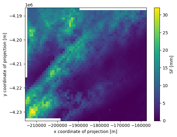
radardays: ['asw 10', 'boo 24', 'drs 24', 'emd 24', 'ess 24', 'fbg ...[12]:
ds_clip.SF.plot()
[12]:
<matplotlib.collections.QuadMesh at 0x7f194f62fad0>
Compute the average precipitation for each catchment#
To compute the zonal average, we have to understand the the grid cells as polygons defined by a set of vertices.
[13]:
# Create vertices for each grid cell
# (MUST BE DONE IN NATIVE RADOLAN COORDINATES)
grid_x, grid_y = np.meshgrid(ds_clip.x, ds_clip.y)
grdverts = wrl.zonalstats.grid_centers_to_vertices(grid_x, grid_y, gridres, gridres)
Create src VectorSource#
This shows how to load data via numpy arrays in a given source projection and project it on the fly to a needed target projection
[14]:
src = wrl.io.VectorSource(
    grdverts, srs=proj_utm, name="src", projection_source=proj_stereo
)
Now we create the ZonalDataPoly class instance providing src and trg VectorSources. Based on the overlap of these polygons with the catchment area, we can then compute a weighted average.
[15]:
# This object collects our source and target data
#   and computes the intersections
zd = wrl.zonalstats.ZonalDataPoly(src, trg, srs=proj_utm)
# zd = wrl.zonalstats.ZonalDataPoly(grdverts, shpfile, srs=proj_utm)

# This object can actually compute the statistics
obj = wrl.zonalstats.ZonalStatsPoly(zd)

# We just call this object with any set of radar data
avg = obj.mean(ds_clip.SF.values.ravel())
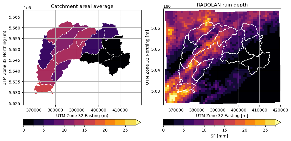
Plot results in map using matplotlib#
We now plot the data using matplotlib accessors of geopandas (vector) and xarray (raster).
[16]:
from matplotlib.colors import from_levels_and_colors

# Create discrete colormap
levels = np.arange(0, 30, 2.5)
colors = pl.cm.inferno(np.linspace(0, 1, len(levels)))
mycmap, mynorm = from_levels_and_colors(levels, colors, extend="max")

fig = pl.figure(figsize=(10, 10))

# Average rainfall sum
ax = fig.add_subplot(121, aspect="equal")
obj.zdata.trg.geo.plot(
    column="mean",
    ax=ax,
    cmap=mycmap,
    norm=mynorm,
    edgecolor="white",
    lw=0.5,
    legend=True,
    legend_kwds=dict(orientation="horizontal", pad=0.05),
)
pl.xlabel("UTM Zone 32 Easting (m)")
pl.ylabel("UTM Zone 32 Northing (m)")
pl.title("Catchment areal average")
bbox = obj.zdata.trg.extent
pl.xlim(bbox[0] - 5000, bbox[1] + 5000)
pl.ylim(bbox[2] - 5000, bbox[3] + 5000)
pl.grid()

# Original radar data
ax = fig.add_subplot(122, aspect="equal")
pm = ds_clip.SF.plot(
    x="xc",
    y="yc",
    cmap=mycmap,
    norm=mynorm,
    ax=ax,
    cbar_kwargs=dict(orientation="horizontal", pad=0.05),
)
obj.zdata.trg.geo.plot(ax=ax, facecolor="None", edgecolor="white")
pl.title("RADOLAN rain depth")
pl.grid(color="white")
pl.tight_layout()
Plot results in interactive map using geopandas#
Interactive mapmaking is easy using geopandas:
[17]:
fmap = obj.zdata.trg.geo.explore(column="mean")
fmap
[17]:
Save time by reading the weights from a file#
The computational expensive part is the computation of intersections and weights. You only need to do it once.
You can dump the results on disk and read them from there when required. Let’s do a little benchmark:
[18]:
import datetime as dt

# dump to file
zd.dump_vector("test_zonal_poly_cart")

t1 = dt.datetime.now()
# Create instance of type ZonalStatsPoly from zonal data file
obj = wrl.zonalstats.ZonalStatsPoly("test_zonal_poly_cart")
t2 = dt.datetime.now()

# Create instance of type ZonalStatsPoly from scratch
src = wrl.io.VectorSource(
    grdverts, srs=proj_utm, name="src", projection_source=proj_stereo
)
trg = wrl.io.VectorSource(shpfile, srs=proj_utm, name="trg")
zd = wrl.zonalstats.ZonalDataPoly(src, trg)
obj = wrl.zonalstats.ZonalStatsPoly(zd)
t3 = dt.datetime.now()

# Calling the object
avg = obj.mean(ds_clip.SF.values.ravel())
t4 = dt.datetime.now()

print("\nCreate object from file: %f seconds" % (t2 - t1).total_seconds())
print("Create object from sratch: %f seconds" % (t3 - t2).total_seconds())
print("Compute stats: %f seconds" % (t4 - t3).total_seconds())
Create object from file: 0.084919 seconds
Create object from sratch: 0.483657 seconds
Compute stats: 0.002049 seconds
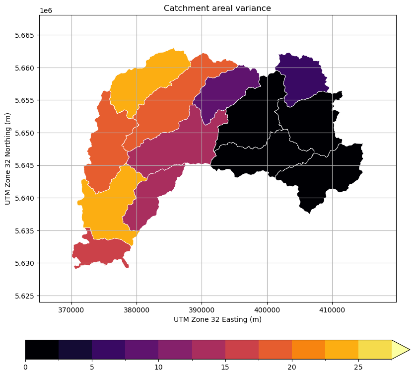
Calculate Variance and Plot Result#
[19]:
var = obj.var(ds_clip.SF.values.ravel())
[20]:
fig = pl.figure(figsize=(10, 10))
ax = fig.add_subplot(111)
obj.zdata.trg.geo.plot(
    column="var",
    ax=ax,
    cmap=mycmap,
    norm=mynorm,
    edgecolor="white",
    lw=0.5,
    legend=True,
    legend_kwds=dict(orientation="horizontal", pad=0.1),
)
pl.xlabel("UTM Zone 32 Easting (m)")
pl.ylabel("UTM Zone 32 Northing (m)")
pl.title("Catchment areal variance")
bbox = obj.zdata.trg.extent
pl.xlim(bbox[0] - 5000, bbox[1] + 5000)
pl.ylim(bbox[2] - 5000, bbox[3] + 5000)
pl.grid()