Plot geodata#

underlay e.g. terrain data from a Digital Elevation Model (DEM)
overlay features such as administrative borders, rivers, catchments, rain gauges, cities, …

Here, we create a map without radar data to concentrate on the other layers.

[1]:

import wradlib as wrl
import matplotlib.pyplot as pl
import warnings

warnings.filterwarnings("ignore")
try:
    get_ipython().run_line_magic("matplotlib inline")
except:
    pl.ion()
import numpy as np

# Some more matplotlib tools we will need...
import matplotlib.ticker as ticker
from matplotlib.colors import LogNorm
from mpl_toolkits.axes_grid1 import make_axes_locatable

/home/runner/micromamba-root/envs/wradlib-tests/lib/python3.11/site-packages/tqdm/auto.py:22: TqdmWarning: IProgress not found. Please update jupyter and ipywidgets. See https://ipywidgets.readthedocs.io/en/stable/user_install.html
  from .autonotebook import tqdm as notebook_tqdm

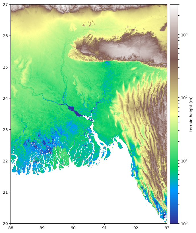
Plotting a Digital Elevation Model (DEM)#

We use a preprocessed geotiff which was created from SRTM data via gdal

gdalwarp -te 88. 20. 93. 27. srtm_54_07.tif srtm_55_07.tif srtm_54_08.tif srtm_55_08.tif bangladesh.tif

Here we - read the DEM via wradlib.io.open_raster and extracted via wradlib.georef.extract_raster_dataset. - resample the data to a (lon/lat) grid with spacing=0.005.

Note: we organise the code in functions which we can re-use in this notebook.

[2]:

def plot_dem(ax):
    filename = wrl.util.get_wradlib_data_file("geo/bangladesh.tif")
    ds = wrl.io.open_raster(filename)
    # pixel_spacing is in output units (lonlat)
    ds = wrl.georef.reproject_raster_dataset(ds, spacing=0.005)
    rastervalues, rastercoords, proj = wrl.georef.extract_raster_dataset(ds)
    # specify kwargs for plotting, using terrain colormap and LogNorm
    dem = ax.pcolormesh(
        rastercoords[..., 0],
        rastercoords[..., 1],
        rastervalues,
        cmap=pl.cm.terrain,
        norm=LogNorm(vmin=1, vmax=3000),
    )
    # make some space on the right for colorbar axis
    div1 = make_axes_locatable(ax)
    cax1 = div1.append_axes("right", size="5%", pad=0.1)
    # add colorbar and title
    # we use LogLocator for colorbar
    cb = pl.gcf().colorbar(dem, cax=cax1, ticks=ticker.LogLocator(subs=range(10)))
    cb.set_label("terrain height [m]")

[3]:

fig = pl.figure(figsize=(10, 10))
ax = fig.add_subplot(111, aspect="equal")
plot_dem(ax)

Downloading file 'geo/bangladesh.tif' from 'https://github.com/wradlib/wradlib-data/raw/pooch/data/geo/bangladesh.tif' to '/home/runner/work/wradlib/wradlib/wradlib-data'.

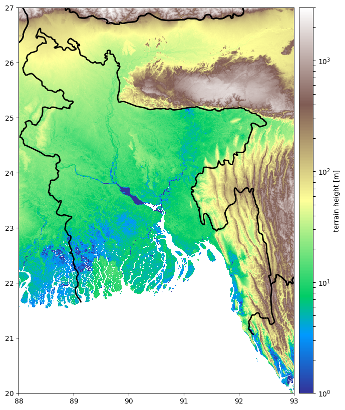
../../_images/notebooks_visualisation_wradlib_overlay_10_1.png

Plotting borders#

For country borders, we use ESRI Shapfiles from Natural Earth Data.

We extract features using - the OGR.Layer AttributeFilter and - the wradlib.georef.get_vector_coordinates function.

The plot overlay is done via wradlib.vis.add_lines.

[4]:

flist = [
    "geo/ne_10m_admin_0_boundary_lines_land.shx",
    "geo/ne_10m_admin_0_boundary_lines_land.prj",
    "geo/ne_10m_admin_0_boundary_lines_land.dbf",
]
[wrl.util.get_wradlib_data_file(f) for f in flist]


def plot_borders(ax):
    # country list
    countries = ["India", "Nepal", "Bhutan", "Myanmar"]
    # open the input data source and get the layer
    filename = wrl.util.get_wradlib_data_file(
        "geo/ne_10m_admin_0_boundary_lines_land.shp"
    )
    dataset, inLayer = wrl.io.open_vector(filename)
    # iterate over countries, filter accordingly, get coordinates and plot
    for item in countries:
        # SQL-like selection syntax
        fattr = "(adm0_left = '" + item + "' or adm0_right = '" + item + "')"
        inLayer.SetAttributeFilter(fattr)
        # get borders and names
        borders, keys = wrl.georef.get_vector_coordinates(inLayer, key="name")
        wrl.vis.add_lines(ax, borders, color="black", lw=2, zorder=4)
    ax.autoscale()

Downloading file 'geo/ne_10m_admin_0_boundary_lines_land.shx' from 'https://github.com/wradlib/wradlib-data/raw/pooch/data/geo/ne_10m_admin_0_boundary_lines_land.shx' to '/home/runner/work/wradlib/wradlib/wradlib-data'.
Downloading file 'geo/ne_10m_admin_0_boundary_lines_land.prj' from 'https://github.com/wradlib/wradlib-data/raw/pooch/data/geo/ne_10m_admin_0_boundary_lines_land.prj' to '/home/runner/work/wradlib/wradlib/wradlib-data'.
Downloading file 'geo/ne_10m_admin_0_boundary_lines_land.dbf' from 'https://github.com/wradlib/wradlib-data/raw/pooch/data/geo/ne_10m_admin_0_boundary_lines_land.dbf' to '/home/runner/work/wradlib/wradlib/wradlib-data'.

[5]:

fig = pl.figure(figsize=(10, 10))
ax = fig.add_subplot(111, aspect="equal")
plot_dem(ax)
plot_borders(ax)
ax.set_xlim((88, 93))
ax.set_ylim((20, 27))

Downloading file 'geo/ne_10m_admin_0_boundary_lines_land.shp' from 'https://github.com/wradlib/wradlib-data/raw/pooch/data/geo/ne_10m_admin_0_boundary_lines_land.shp' to '/home/runner/work/wradlib/wradlib/wradlib-data'.

[5]:

(20.0, 27.0)

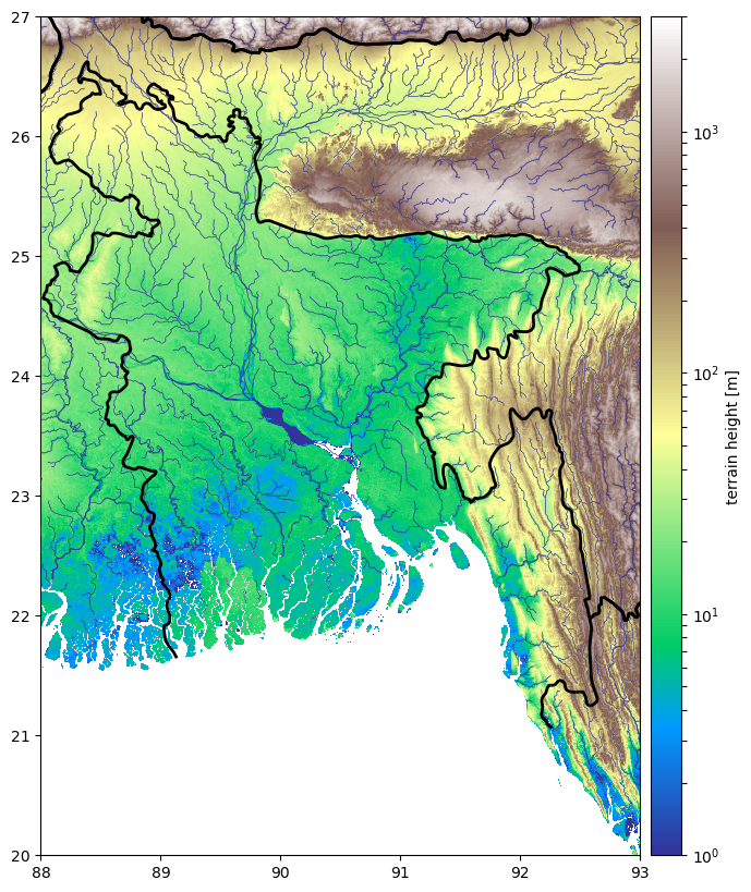
../../_images/notebooks_visualisation_wradlib_overlay_15_2.png

Plotting Rivers#

For rivers, we use ESRI Shapfiles from FAO and Natural Earth Data.

We extract features using - the OGR.Layer SpatialFilter and - the wradlib.georef.get_vector_coordinates function.

Then we use wradlib.vis.add_lines again for the overlay.

[6]:

flist = [
    "geo/rivers_asia_37331.shx",
    "geo/rivers_asia_37331.prj",
    "geo/rivers_asia_37331.dbf",
]
[wrl.util.get_wradlib_data_file(f) for f in flist]


def plot_rivers(ax):
    # plot rivers from esri vector shape, filter spatially
    # http://www.fao.org/geonetwork/srv/en/metadata.show?id=37331

    # open the input data source and get the layer
    filename = wrl.util.get_wradlib_data_file("geo/rivers_asia_37331.shp")
    dataset, inLayer = wrl.io.open_vector(filename)

    # do spatial filtering to get only geometries inside bounding box
    inLayer.SetSpatialFilterRect(88, 20, 93, 27)
    rivers, keys = wrl.georef.get_vector_coordinates(inLayer, key="MAJ_NAME")

    # plot on ax1, and ax4
    wrl.vis.add_lines(ax, rivers, color=pl.cm.terrain(0.0), lw=0.5, zorder=3)

Downloading file 'geo/rivers_asia_37331.shx' from 'https://github.com/wradlib/wradlib-data/raw/pooch/data/geo/rivers_asia_37331.shx' to '/home/runner/work/wradlib/wradlib/wradlib-data'.
Downloading file 'geo/rivers_asia_37331.prj' from 'https://github.com/wradlib/wradlib-data/raw/pooch/data/geo/rivers_asia_37331.prj' to '/home/runner/work/wradlib/wradlib/wradlib-data'.
Downloading file 'geo/rivers_asia_37331.dbf' from 'https://github.com/wradlib/wradlib-data/raw/pooch/data/geo/rivers_asia_37331.dbf' to '/home/runner/work/wradlib/wradlib/wradlib-data'.

[7]:

fig = pl.figure(figsize=(10, 10))
ax = fig.add_subplot(111, aspect="equal")
plot_dem(ax)
plot_borders(ax)
plot_rivers(ax)
ax.set_xlim((88, 93))
ax.set_ylim((20, 27))

Downloading file 'geo/rivers_asia_37331.shp' from 'https://github.com/wradlib/wradlib-data/raw/pooch/data/geo/rivers_asia_37331.shp' to '/home/runner/work/wradlib/wradlib/wradlib-data'.

[7]:

(20.0, 27.0)

../../_images/notebooks_visualisation_wradlib_overlay_20_2.png

[8]:

flist = [
    "geo/ne_10m_rivers_lake_centerlines.shx",
    "geo/ne_10m_rivers_lake_centerlines.prj",
    "geo/ne_10m_rivers_lake_centerlines.dbf",
]
[wrl.util.get_wradlib_data_file(f) for f in flist]


def plot_water(ax):
    # plot rivers from esri vector shape, filter spatially
    # plot rivers from NED
    # open the input data source and get the layer
    filename = wrl.util.get_wradlib_data_file("geo/ne_10m_rivers_lake_centerlines.shp")
    dataset, inLayer = wrl.io.open_vector(filename)
    inLayer.SetSpatialFilterRect(88, 20, 93, 27)
    rivers, keys = wrl.georef.get_vector_coordinates(inLayer)
    wrl.vis.add_lines(ax, rivers, color=pl.cm.terrain(0.0), lw=0.5, zorder=3)

Downloading file 'geo/ne_10m_rivers_lake_centerlines.shx' from 'https://github.com/wradlib/wradlib-data/raw/pooch/data/geo/ne_10m_rivers_lake_centerlines.shx' to '/home/runner/work/wradlib/wradlib/wradlib-data'.
Downloading file 'geo/ne_10m_rivers_lake_centerlines.prj' from 'https://github.com/wradlib/wradlib-data/raw/pooch/data/geo/ne_10m_rivers_lake_centerlines.prj' to '/home/runner/work/wradlib/wradlib/wradlib-data'.
Downloading file 'geo/ne_10m_rivers_lake_centerlines.dbf' from 'https://github.com/wradlib/wradlib-data/raw/pooch/data/geo/ne_10m_rivers_lake_centerlines.dbf' to '/home/runner/work/wradlib/wradlib/wradlib-data'.

[9]:

fig = pl.figure(figsize=(10, 10))
ax = fig.add_subplot(111, aspect="equal")
plot_dem(ax)
plot_borders(ax)
plot_rivers(ax)
plot_water(ax)
ax.set_xlim((88, 93))
ax.set_ylim((20, 27))

Downloading file 'geo/ne_10m_rivers_lake_centerlines.shp' from 'https://github.com/wradlib/wradlib-data/raw/pooch/data/geo/ne_10m_rivers_lake_centerlines.shp' to '/home/runner/work/wradlib/wradlib/wradlib-data'.

[9]:

(20.0, 27.0)

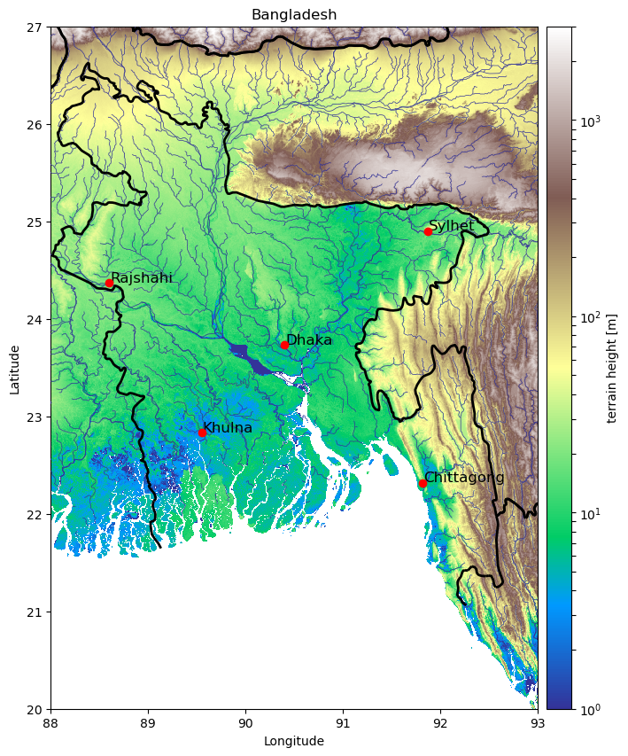
../../_images/notebooks_visualisation_wradlib_overlay_22_2.png

Plotting Cities#

The 5 biggest cities of bangladesh are added using simple matplotlib functions.

[10]:

def plot_cities(ax):
    # plot city dots with annotation, finalize plot
    # lat/lon coordinates of five cities in Bangladesh
    lats = [23.73, 22.32, 22.83, 24.37, 24.90]
    lons = [90.40, 91.82, 89.55, 88.60, 91.87]
    cities = ["Dhaka", "Chittagong", "Khulna", "Rajshahi", "Sylhet"]
    for lon, lat, city in zip(lons, lats, cities):
        ax.plot(lon, lat, "ro", zorder=5)
        ax.text(lon + 0.01, lat + 0.01, city, fontsize="large")

[11]:

fig = pl.figure(figsize=(10, 10))
ax = fig.add_subplot(111, aspect="equal")
plot_dem(ax)
plot_borders(ax)
plot_rivers(ax)
plot_water(ax)
plot_cities(ax)

ax.set_xlim((88, 93))
ax.set_ylim((20, 27))
ax.set_xlabel("Longitude")
ax.set_ylabel("Latitude")
ax.set_aspect("equal")
ax.set_title("Bangladesh")

[11]:

Text(0.5, 1.0, 'Bangladesh')

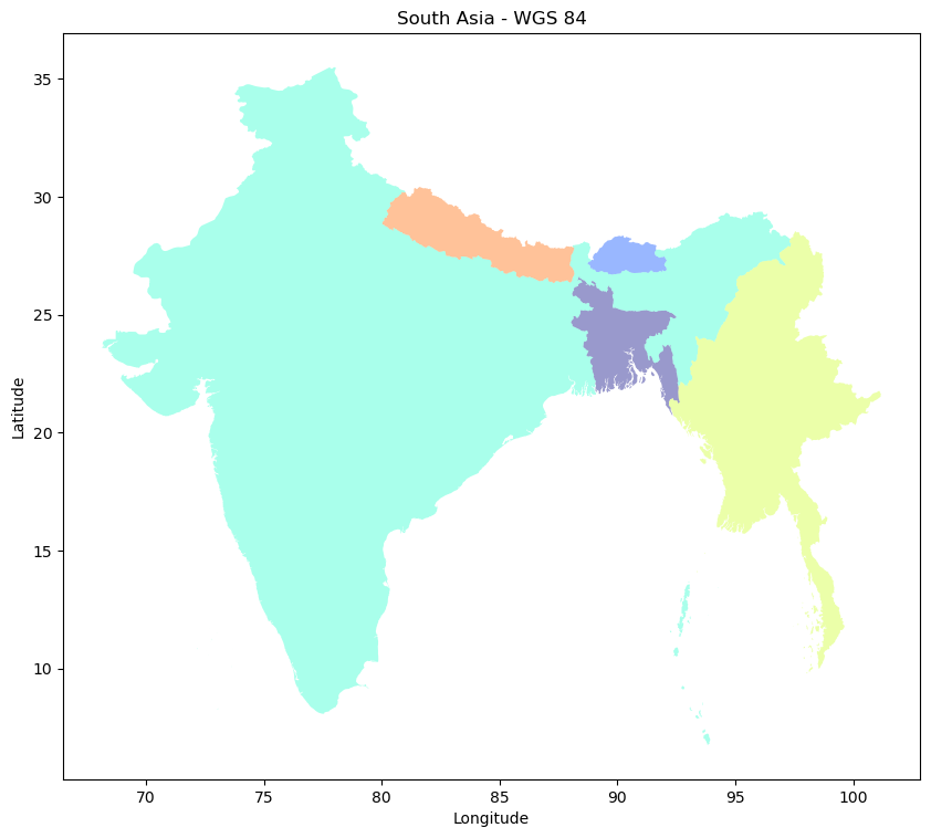
../../_images/notebooks_visualisation_wradlib_overlay_26_1.png

Plotting country patches#

Plotting in “geographic projection” (WGS84)#

Here, we plot countries as patches on a lat/lon (WGS84) map (data from Natural Earth Data again).

We again extract the features using - the OGR.Layer SpatialFilter and - wradlib.georef.get_vector_coordinates.

Then the patches are added one by one via wradlib.vis.add_patches.

[12]:

flist = [
    "geo/ne_10m_admin_0_countries.shx",
    "geo/ne_10m_admin_0_countries.prj",
    "geo/ne_10m_admin_0_countries.dbf",
]
[wrl.util.get_wradlib_data_file(f) for f in flist]


def plot_wgs84(ax):
    from osgeo import osr

    wgs84 = osr.SpatialReference()
    wgs84.ImportFromEPSG(4326)
    # some testing on additional axes
    # add Bangladesh to countries
    countries = ["India", "Nepal", "Bhutan", "Myanmar", "Bangladesh"]
    # create colors for country-patches
    cm = pl.cm.jet
    colors = []
    for i in range(len(countries)):
        colors.append(cm(1.0 * i / len(countries)))

    # open the input data source and get the layer
    filename = wrl.util.get_wradlib_data_file("geo/ne_10m_admin_0_countries.shp")
    dataset, layer = wrl.io.open_vector(filename)

    # filter spatially and plot as PatchCollection on ax3
    layer.SetSpatialFilterRect(88, 20, 93, 27)
    patches, keys = wrl.georef.get_vector_coordinates(layer, dest_srs=wgs84, key="name")
    i = 0
    for name, patch in zip(keys, patches):
        # why comes the US in here?
        if name in countries:
            wrl.vis.add_patches(
                ax, patch, facecolor=colors[i], cmap=pl.cm.viridis, alpha=0.4
            )
            i += 1
    ax.autoscale(True)
    ax.set_aspect("equal")
    ax.set_xlabel("Longitude")
    ax.set_ylabel("Latitude")
    ax.set_title("South Asia - WGS 84")

Downloading file 'geo/ne_10m_admin_0_countries.shx' from 'https://github.com/wradlib/wradlib-data/raw/pooch/data/geo/ne_10m_admin_0_countries.shx' to '/home/runner/work/wradlib/wradlib/wradlib-data'.
Downloading file 'geo/ne_10m_admin_0_countries.prj' from 'https://github.com/wradlib/wradlib-data/raw/pooch/data/geo/ne_10m_admin_0_countries.prj' to '/home/runner/work/wradlib/wradlib/wradlib-data'.
Downloading file 'geo/ne_10m_admin_0_countries.dbf' from 'https://github.com/wradlib/wradlib-data/raw/pooch/data/geo/ne_10m_admin_0_countries.dbf' to '/home/runner/work/wradlib/wradlib/wradlib-data'.

[13]:

fig = pl.figure(figsize=(10, 10))
ax = fig.add_subplot(111, aspect="equal")
plot_wgs84(ax)

Downloading file 'geo/ne_10m_admin_0_countries.shp' from 'https://github.com/wradlib/wradlib-data/raw/pooch/data/geo/ne_10m_admin_0_countries.shp' to '/home/runner/work/wradlib/wradlib/wradlib-data'.

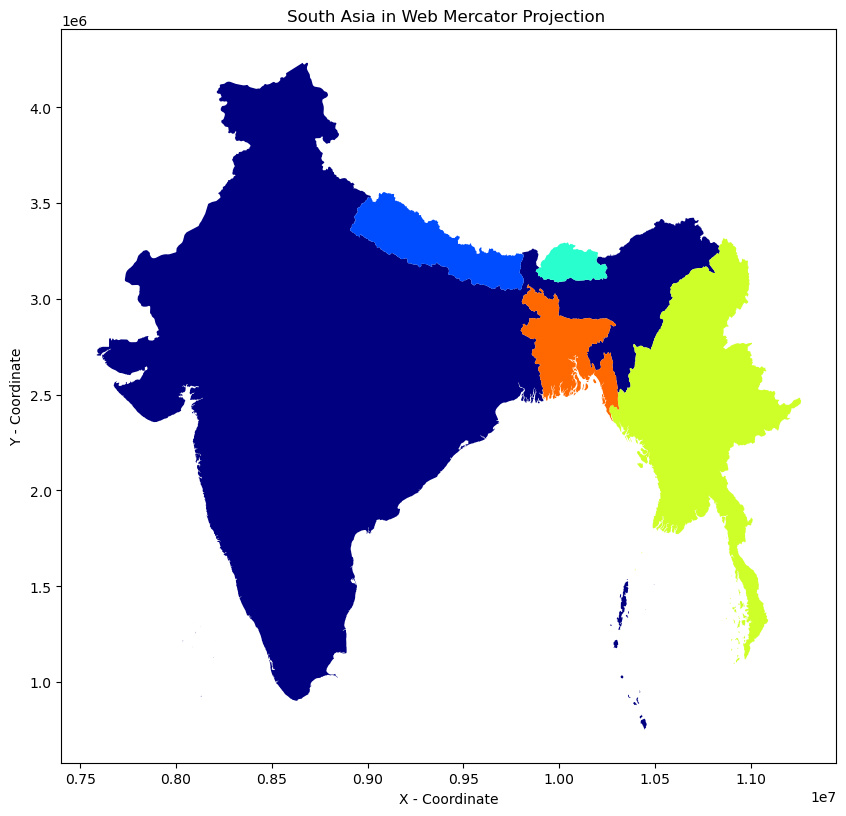
../../_images/notebooks_visualisation_wradlib_overlay_33_1.png

Plotting with a map projection#

Here, we plot countries as patches on a projected map.

We extract the features using - the OGR.Layer AttributeFilter and - the wradlib.georef.get_vector_coordinates function.

The coordinates of the features are reprojected on the fly using the dest_srs keyword of wradlib.georef.get_vector_coordinates.

Then, the patches are added to the map via wradlib.vis.add_patches.

[14]:

def plot_mercator(ax):
    from osgeo import osr

    proj = osr.SpatialReference()
    # "Web Mercator" projection (used by GoogleMaps, OSM, ...)
    proj.ImportFromEPSG(3857)

    # add Bangladesh to countries
    countries = ["India", "Nepal", "Bhutan", "Myanmar", "Bangladesh"]
    # create colors for country-patches
    cm = pl.cm.jet
    colors = []
    for i in range(len(countries)):
        colors.append(cm(1.0 * i / len(countries)))

    # open the input data source and get the layer
    filename = wrl.util.get_wradlib_data_file("geo/ne_10m_admin_0_countries.shp")
    dataset, layer = wrl.io.open_vector(filename)
    # iterate over countries, filter by attribute,
    # plot single patches on ax2
    for i, item in enumerate(countries):
        fattr = "name = '" + item + "'"
        layer.SetAttributeFilter(fattr)
        # get country patches and geotransform to destination srs
        patches, keys = wrl.georef.get_vector_coordinates(
            layer, dest_srs=proj, key="name"
        )
        wrl.vis.add_patches(pl.gca(), patches, facecolor=colors[i])

    ax.autoscale(True)
    ax.set_aspect("equal")
    ax.set_xlabel("X - Coordinate")
    ax.set_ylabel("Y - Coordinate")
    ax.ticklabel_format(style="sci", scilimits=(0, 0))
    ax.set_title("South Asia in Web Mercator Projection ")

[15]:

fig = pl.figure(figsize=(10, 10))
ax = fig.add_subplot(111, aspect="equal")
plot_mercator(ax)

../../_images/notebooks_visualisation_wradlib_overlay_39_0.png

Plot geodata

Contents