Plotting Radar Scan Strategy#
This notebook shows how to plot the scan strategy of a specific radar.
[1]:
import wradlib as wrl
import matplotlib.pyplot as pl
import matplotlib as mpl
import warnings

warnings.filterwarnings("ignore")
try:
    get_ipython().run_line_magic("matplotlib inline")
except:
    pl.ion()
import numpy as np
/home/runner/micromamba-root/envs/wradlib-tests/lib/python3.11/site-packages/tqdm/auto.py:22: TqdmWarning: IProgress not found. Please update jupyter and ipywidgets. See https://ipywidgets.readthedocs.io/en/stable/user_install.html
  from .autonotebook import tqdm as notebook_tqdm
Setup Radar details#
[2]:
nrays = 360
nbins = 150
range_res = 500.0
ranges = np.arange(nbins) * range_res
elevs = [28.0, 18.0, 14.0, 11.0, 8.2, 6.0, 4.5, 3.1, 2.0, 1.0]
sitecoords = (-28.1, 38.42, 450.0)
beamwidth = 1.0
Standard Plot#
This works with some assumptions:
beamwidth = 1.0
vert_res = 500.0
maxalt = 10000.0
units = ‘m’
[3]:
ax = wrl.vis.plot_scan_strategy(ranges, elevs, sitecoords)
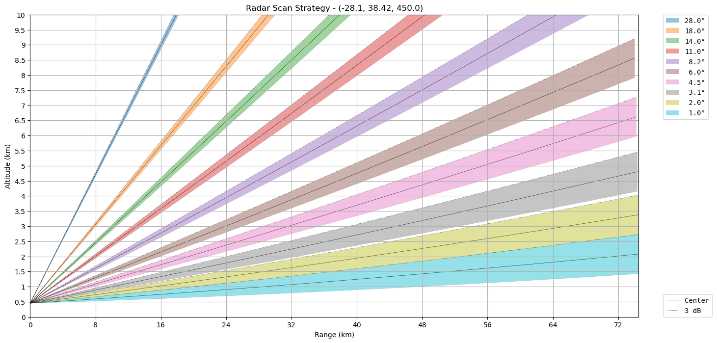
Change Plot Style#
Plot Axes in Kilometer#
To quickly change the Axes tickmarks and labels from meter to kilometer, just add keyword argument units='km'.
[4]:
ax = wrl.vis.plot_scan_strategy(ranges, elevs, sitecoords, units="km")
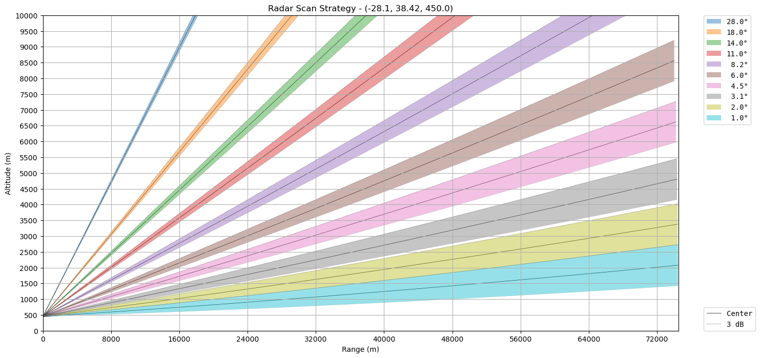
Change Axes Resolution and Range#
The horizontal and vertical Axes Resolution and Range can be set by feeding keyword arguments vert_res, maxalt, range_res, max_range in meter.
[5]:
ax = wrl.vis.plot_scan_strategy(
    ranges,
    elevs,
    sitecoords,
    vert_res=1000.0,
    maxalt=15000.0,
    range_res=5000.0,
    maxrange=75000.0,
    units="km",
)

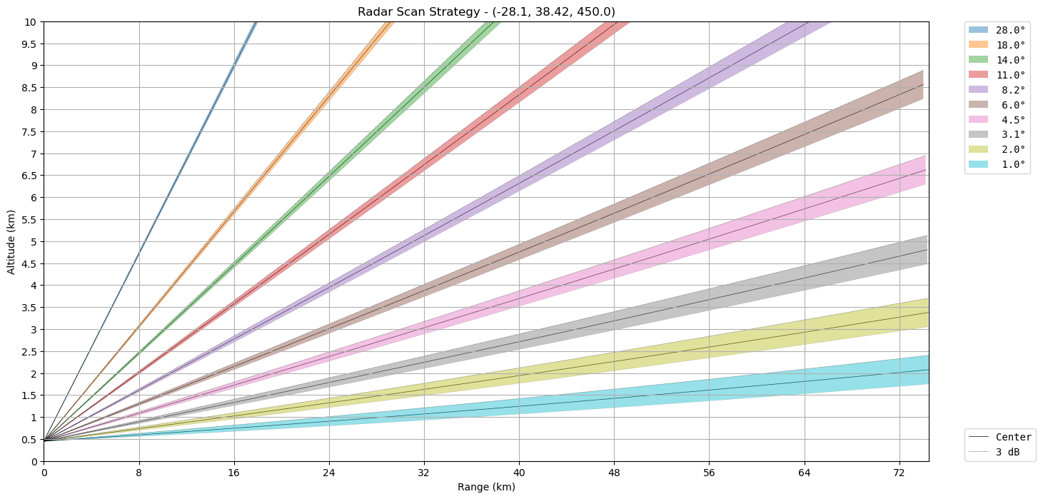
Change Beamwidth#
The beamwidth defaults to 1.0°. It can specified by keyword argument beamwidth.
[6]:
ax = wrl.vis.plot_scan_strategy(ranges, elevs, sitecoords, beamwidth=0.5, units="km")
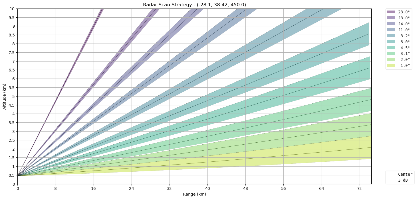
Change Colors#
The colorcycle can be changed from the default tab10 to any colormap available in matplotlib. If the output is intended to be plotted as grey-scale, the use of the Perceptually Uniform Sequential colormaps (eg. viridis, cividis) is suggested.
[7]:
ax = wrl.vis.plot_scan_strategy(ranges, elevs, sitecoords, units="km", cmap="viridis")
Plot Terrain#
A terrain profile can be added to the plot by specifying keyword argument terrain=True which automatically downloads neccessary SRTM DEM data and calculates the terrain profile. Additionally the azimuth angle need to be set via keyword argument az (it would default to 0, pointing due north).
For this to work the WRADLIB_DATA environment variable has to point a writable folder. Aditionally users need an earthdata account with bearer token.
[8]:
# only run if environment variables are set
import os

has_data = os.environ.get("WRADLIB_EARTHDATA_BEARER_TOKEN", False)
[9]:
if has_data:
    ax = wrl.vis.plot_scan_strategy(
        ranges, elevs, sitecoords, units="km", terrain=True, az=10
    )
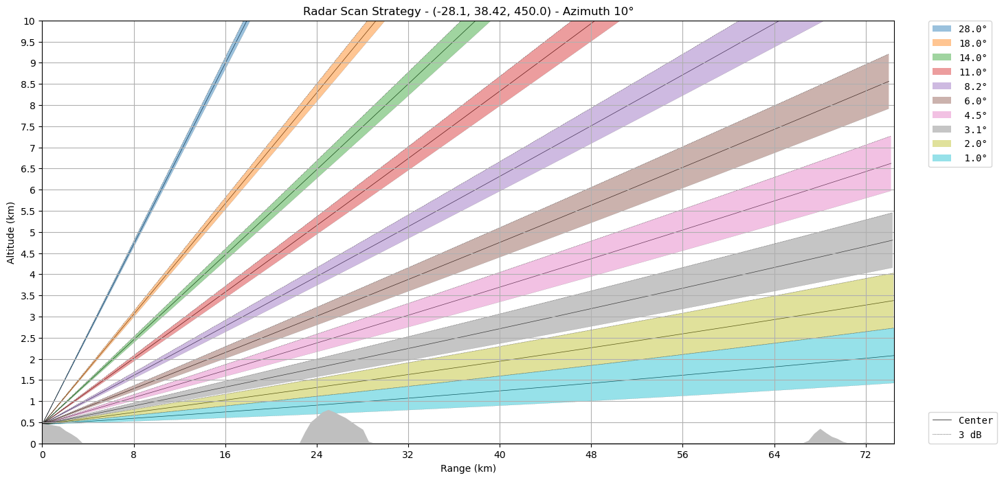
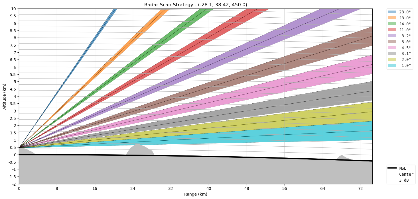
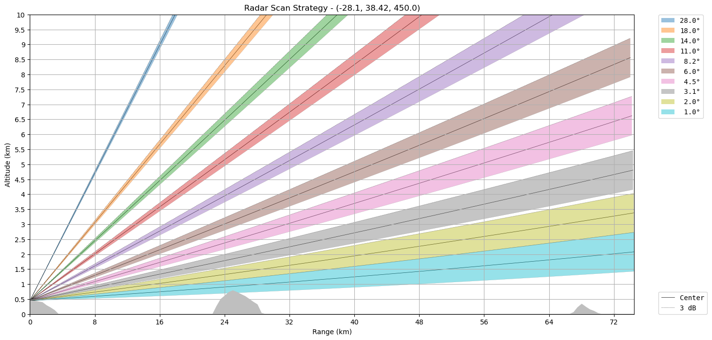
Instead of downloading the SRTM data a precomputed terrain profile can be plotted. Just for the purpose to show this, the terrain data is calculated via the same mechanism as in plot_scan_strategy. The profile should be fed via the same keyword argument terrain.
[10]:
flist = [
    "geo/N38W028.SRTMGL3.hgt.zip",
    "geo/N38W029.SRTMGL3.hgt.zip",
    "geo/N39W028.SRTMGL3.hgt.zip",
    "geo/N39W029.SRTMGL3.hgt.zip",
]
[wrl.util.get_wradlib_data_file(f) for f in flist]
xyz, rad = wrl.georef.spherical_to_xyz(ranges, [10.0], elevs, sitecoords, squeeze=True)
ll = wrl.georef.reproject(xyz, projection_source=rad)

# (down-)load srtm data
ds = wrl.io.get_srtm(
    [ll[..., 0].min(), ll[..., 0].max(), ll[..., 1].min(), ll[..., 1].max()],
)
rastervalues, rastercoords, proj = wrl.georef.extract_raster_dataset(
    ds, nodata=-32768.0
)
# map rastervalues to polar grid points
terrain = wrl.ipol.cart_to_irregular_spline(
    rastercoords, rastervalues, ll[-1, ..., :2], order=3, prefilter=False
)
[11]:
ax = wrl.vis.plot_scan_strategy(ranges, elevs, sitecoords, units="km", terrain=terrain)
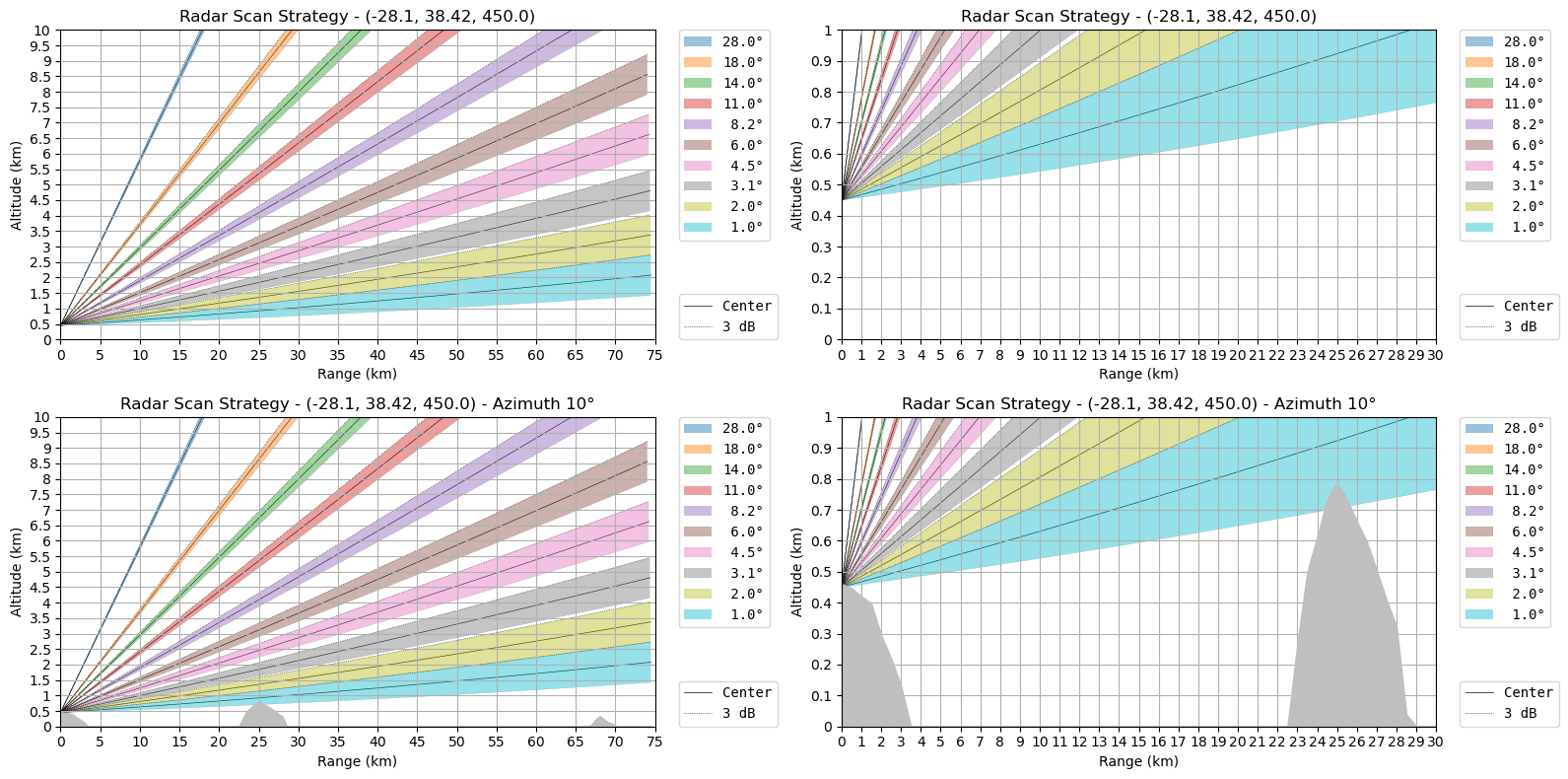
Plotting in grids#
The keyword argument ax can be used to specify the axes to plot in.
[12]:
if has_data:
    fig = pl.figure(figsize=(16, 8))
    ax1 = 221
    ax1 = wrl.vis.plot_scan_strategy(
        ranges,
        elevs,
        sitecoords,
        beamwidth=1.0,
        vert_res=500.0,
        range_res=5000.0,
        maxrange=75000.0,
        units="km",
        terrain=None,
        ax=ax1,
    )
    ax2 = 222
    ax2 = wrl.vis.plot_scan_strategy(
        ranges,
        elevs,
        sitecoords,
        beamwidth=1.0,
        vert_res=100.0,
        maxalt=1000.0,
        range_res=1000.0,
        maxrange=30000.0,
        units="km",
        terrain=None,
        ax=ax2,
    )
    ax3 = 223
    ax3 = wrl.vis.plot_scan_strategy(
        ranges,
        elevs,
        sitecoords,
        beamwidth=1.0,
        vert_res=500.0,
        range_res=5000.0,
        maxrange=75000.0,
        units="km",
        terrain=True,
        az=10,
        ax=ax3,
    )
    ax4 = 224
    ax4 = wrl.vis.plot_scan_strategy(
        ranges,
        elevs,
        sitecoords,
        beamwidth=1.0,
        vert_res=100.0,
        maxalt=1000.0,
        range_res=1000.0,
        maxrange=30000.0,
        units="km",
        terrain=True,
        az=10,
        ax=ax4,
    )
    pl.tight_layout()
Plotting with curvelinear grid#
All of the above shown plotting into a cartesian coordinate system is also possible with a curvelinear grid. Just set keyword argument cg=True. The thick black line denotes the earth mean sea level (MSL).
[13]:
ax = wrl.vis.plot_scan_strategy(
    ranges, elevs, sitecoords, units="km", cg=True, terrain=terrain
)