How to use wradlib’s ipol module for interpolation tasks?#
[1]:
import wradlib.ipol as ipol
from wradlib.util import get_wradlib_data_file
from wradlib.vis import plot_ppi
import numpy as np
import matplotlib.pyplot as pl
import datetime as dt
import warnings

warnings.filterwarnings("ignore")
try:
    get_ipython().run_line_magic("matplotlib inline")
except:
    pl.ion()
/home/runner/micromamba-root/envs/wradlib-tests/lib/python3.11/site-packages/tqdm/auto.py:22: TqdmWarning: IProgress not found. Please update jupyter and ipywidgets. See https://ipywidgets.readthedocs.io/en/stable/user_install.html
  from .autonotebook import tqdm as notebook_tqdm
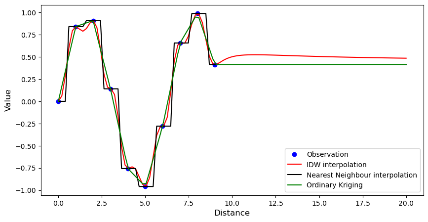
1-dimensional example#
Includes Nearest Neighbours, Inverse Distance Weighting, and Ordinary Kriging.
[2]:
# Synthetic observations
xsrc = np.arange(10)[:, None]
vals = np.sin(xsrc).ravel()

# Define target coordinates
xtrg = np.linspace(0, 20, 100)[:, None]

# Set up interpolation objects
#   IDW
idw = ipol.Idw(xsrc, xtrg)
#   Nearest Neighbours
nn = ipol.Nearest(xsrc, xtrg)
#   Linear
ok = ipol.OrdinaryKriging(xsrc, xtrg)

# Plot results
pl.figure(figsize=(10, 5))
pl.plot(xsrc.ravel(), vals, "bo", label="Observation")
pl.plot(xtrg.ravel(), idw(vals), "r-", label="IDW interpolation")
pl.plot(xtrg.ravel(), nn(vals), "k-", label="Nearest Neighbour interpolation")
pl.plot(xtrg.ravel(), ok(vals), "g-", label="Ordinary Kriging")
pl.xlabel("Distance", fontsize="large")
pl.ylabel("Value", fontsize="large")
pl.legend(loc="lower right")
[2]:
<matplotlib.legend.Legend at 0x7f1d97ecd050>
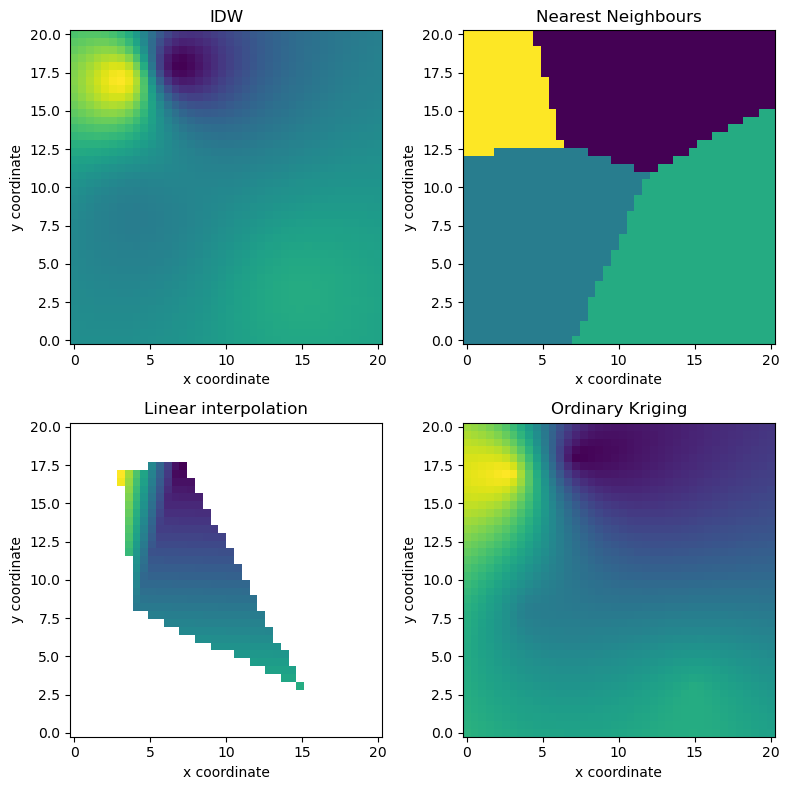
2-dimensional example#
Includes Nearest Neighbours, Inverse Distance Weighting, Linear Interpolation, and Ordinary Kriging.
[3]:
# Synthetic observations and source coordinates
src = np.vstack((np.array([4, 7, 3, 15]), np.array([8, 18, 17, 3]))).transpose()
np.random.seed(1319622840)
vals = np.random.uniform(size=len(src))

# Target coordinates
xtrg = np.linspace(0, 20, 40)
ytrg = np.linspace(0, 20, 40)
trg = np.meshgrid(xtrg, ytrg)
trg = np.vstack((trg[0].ravel(), trg[1].ravel())).T

# Interpolation objects
idw = ipol.Idw(src, trg)
nn = ipol.Nearest(src, trg)
linear = ipol.Linear(src, trg)
ok = ipol.OrdinaryKriging(src, trg)


# Subplot layout
def gridplot(interpolated, title=""):
    pm = ax.pcolormesh(xtrg, ytrg, interpolated.reshape((len(xtrg), len(ytrg))))
    pl.axis("tight")
    ax.scatter(src[:, 0], src[:, 1], facecolor="None", s=50, marker="s")
    pl.title(title)
    pl.xlabel("x coordinate")
    pl.ylabel("y coordinate")


# Plot results
fig = pl.figure(figsize=(8, 8))
ax = fig.add_subplot(221, aspect="equal")
gridplot(idw(vals), "IDW")
ax = fig.add_subplot(222, aspect="equal")
gridplot(nn(vals), "Nearest Neighbours")
ax = fig.add_subplot(223, aspect="equal")
gridplot(np.ma.masked_invalid(linear(vals)), "Linear interpolation")
ax = fig.add_subplot(224, aspect="equal")
gridplot(ok(vals), "Ordinary Kriging")
pl.tight_layout()
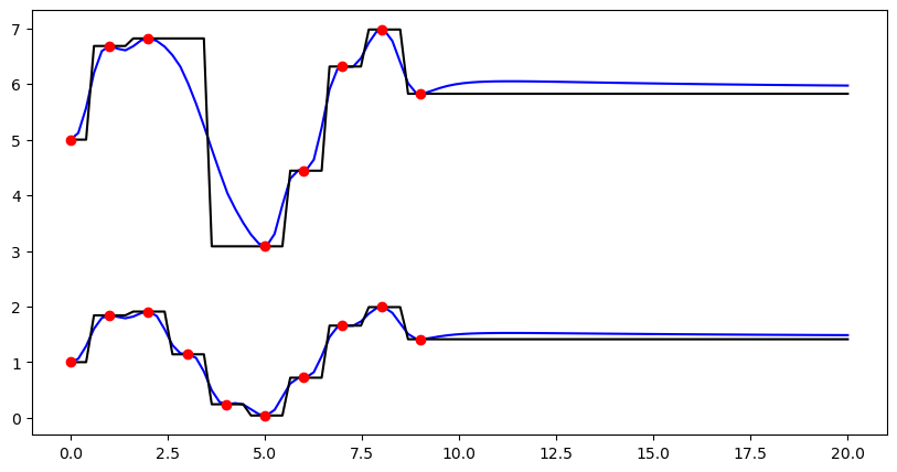
Using the convenience function ipol.interpolation in order to deal with missing values#
(1) Exemplified for one dimension in space and two dimensions of the source value array (could e.g. be two time steps).
[4]:
# Synthetic observations (e.g. two time steps)
src = np.arange(10)[:, None]
vals = np.hstack((1.0 + np.sin(src), 5.0 + 2.0 * np.sin(src)))
# Target coordinates
trg = np.linspace(0, 20, 100)[:, None]
# Here we introduce missing values in the second dimension of the source value array
vals[3:5, 1] = np.nan
# interpolation using the convenience function "interpolate"
idw_result = ipol.interpolate(src, trg, vals, ipol.Idw, nnearest=4)
nn_result = ipol.interpolate(src, trg, vals, ipol.Nearest)
# Plot results
fig = pl.figure(figsize=(10, 5))
ax = fig.add_subplot(111)
pl1 = ax.plot(trg, idw_result, "b-", label="IDW")
pl2 = ax.plot(trg, nn_result, "k-", label="Nearest Neighbour")
pl3 = ax.plot(src, vals, "ro", label="Observations")
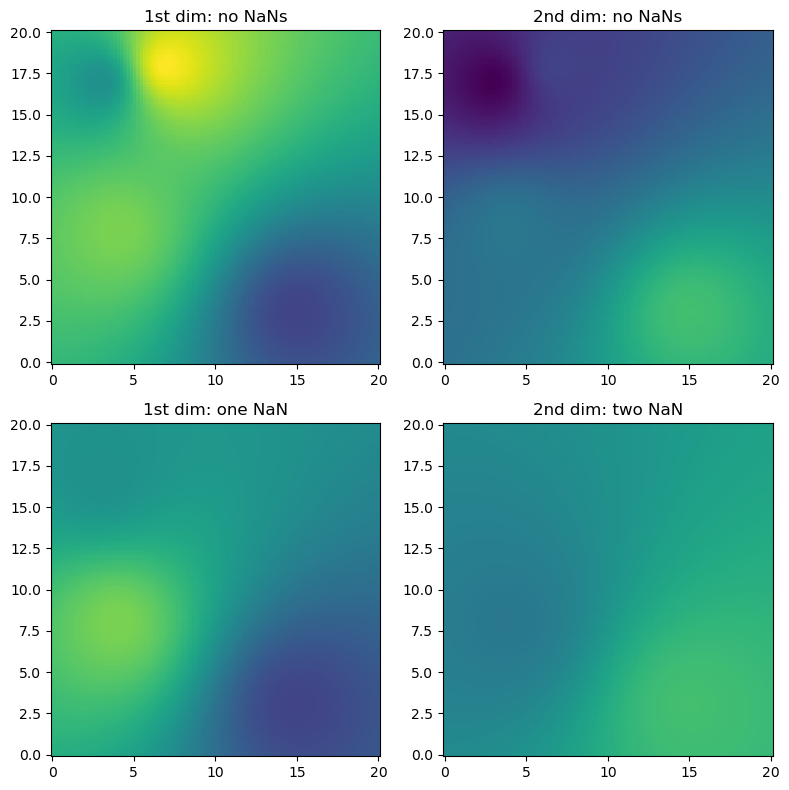
(2) Exemplified for two dimensions in space and two dimensions of the source value array (e.g. time steps), containing also NaN values (here we only use IDW interpolation)
[5]:
# Just a helper function for repeated subplots
def plotall(ax, trgx, trgy, src, interp, pts, title, vmin, vmax):
    ix = np.where(np.isfinite(pts))
    ax.pcolormesh(
        trgx, trgy, interp.reshape((len(trgx), len(trgy))), vmin=vmin, vmax=vmax
    )
    ax.scatter(
        src[ix, 0].ravel(),
        src[ix, 1].ravel(),
        c=pts.ravel()[ix],
        s=20,
        marker="s",
        vmin=vmin,
        vmax=vmax,
    )
    ax.set_title(title)
    pl.axis("tight")
[6]:
# Synthetic observations
src = np.vstack((np.array([4, 7, 3, 15]), np.array([8, 18, 17, 3]))).T
np.random.seed(1319622840 + 1)
vals = np.round(np.random.uniform(size=(len(src), 2)), 1)

# Target coordinates
trgx = np.linspace(0, 20, 100)
trgy = np.linspace(0, 20, 100)
trg = np.meshgrid(trgx, trgy)
trg = np.vstack((trg[0].ravel(), trg[1].ravel())).transpose()

result = ipol.interpolate(src, trg, vals, ipol.Idw, nnearest=4)

# Now introduce NaNs in the observations
vals_with_nan = vals.copy()
vals_with_nan[1, 0] = np.nan
vals_with_nan[1:3, 1] = np.nan
result_with_nan = ipol.interpolate(src, trg, vals_with_nan, ipol.Idw, nnearest=4)
vmin = np.concatenate((vals.ravel(), result.ravel())).min()
vmax = np.concatenate((vals.ravel(), result.ravel())).max()

fig = pl.figure(figsize=(8, 8))
ax = fig.add_subplot(221)
plotall(ax, trgx, trgy, src, result[:, 0], vals[:, 0], "1st dim: no NaNs", vmin, vmax)
ax = fig.add_subplot(222)
plotall(ax, trgx, trgy, src, result[:, 1], vals[:, 1], "2nd dim: no NaNs", vmin, vmax)
ax = fig.add_subplot(223)
plotall(
    ax,
    trgx,
    trgy,
    src,
    result_with_nan[:, 0],
    vals_with_nan[:, 0],
    "1st dim: one NaN",
    vmin,
    vmax,
)
ax = fig.add_subplot(224)
plotall(
    ax,
    trgx,
    trgy,
    src,
    result_with_nan[:, 1],
    vals_with_nan[:, 1],
    "2nd dim: two NaN",
    vmin,
    vmax,
)
pl.tight_layout()
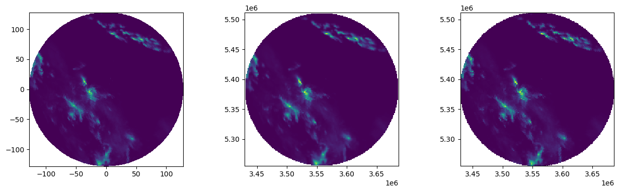
How to use interpolation for gridding data in polar coordinates?#
Read polar coordinates and corresponding rainfall intensity from file
[7]:
filename = get_wradlib_data_file("misc/bin_coords_tur.gz")
src = np.loadtxt(filename)

filename = get_wradlib_data_file("misc/polar_R_tur.gz")
vals = np.loadtxt(filename)
Downloading file 'misc/bin_coords_tur.gz' from 'https://github.com/wradlib/wradlib-data/raw/pooch/data/misc/bin_coords_tur.gz' to '/home/runner/work/wradlib/wradlib/wradlib-data'.
Downloading file 'misc/polar_R_tur.gz' from 'https://github.com/wradlib/wradlib-data/raw/pooch/data/misc/polar_R_tur.gz' to '/home/runner/work/wradlib/wradlib/wradlib-data'.
[8]:
src.shape
[8]:
(46080, 2)
Define target grid coordinates
[9]:
xtrg = np.linspace(src[:, 0].min(), src[:, 0].max(), 200)
ytrg = np.linspace(src[:, 1].min(), src[:, 1].max(), 200)
trg = np.meshgrid(xtrg, ytrg)
trg = np.vstack((trg[0].ravel(), trg[1].ravel())).T
Linear Interpolation
[10]:
ip_lin = ipol.Linear(src, trg)
result_lin = ip_lin(vals.ravel(), fill_value=np.nan)
IDW interpolation
[11]:
ip_near = ipol.Nearest(src, trg)
maxdist = trg[1, 0] - trg[0, 0]
result_near = ip_near(vals.ravel(), maxdist=maxdist)
Plot results
[12]:
fig = pl.figure(figsize=(15, 6))
fig.subplots_adjust(wspace=0.4)
ax = fig.add_subplot(131, aspect="equal")
plot_ppi(vals, ax=ax)
ax = fig.add_subplot(132, aspect="equal")
pl.pcolormesh(xtrg, ytrg, result_lin.reshape((len(xtrg), len(ytrg))))
ax = fig.add_subplot(133, aspect="equal")
pl.pcolormesh(xtrg, ytrg, result_near.reshape((len(xtrg), len(ytrg))))
[12]:
<matplotlib.collections.QuadMesh at 0x7f1d9404f490>