Heuristic clutter detection based on distribution properties (“histo cut”)#
Detects areas with anomalously low or high average reflectivity or precipitation. It is recommended to use long term average or sums (months to year).
[1]:
import wradlib.clutter as clutter
from wradlib.vis import plot_ppi
import wradlib.util as util
import numpy as np
import matplotlib.pyplot as pl
import warnings

warnings.filterwarnings("ignore")
try:
    get_ipython().run_line_magic("matplotlib inline")
except:
    pl.ion()
/home/runner/micromamba-root/envs/wradlib-tests/lib/python3.11/site-packages/tqdm/auto.py:22: TqdmWarning: IProgress not found. Please update jupyter and ipywidgets. See https://ipywidgets.readthedocs.io/en/stable/user_install.html
  from .autonotebook import tqdm as notebook_tqdm
Load annual rainfall acummulation example (from DWD radar Feldberg)#
[2]:
filename = util.get_wradlib_data_file("misc/annual_rainfall_fbg.gz")
yearsum = np.loadtxt(filename)
Downloading file 'misc/annual_rainfall_fbg.gz' from 'https://github.com/wradlib/wradlib-data/raw/pooch/data/misc/annual_rainfall_fbg.gz' to '/home/runner/work/wradlib/wradlib/wradlib-data'.
Apply histo-cut filter to retrieve boolean array that highlights clutter as well as beam blockage#
Depending on your data and climate you can parameterize the upper and lower frequency percentage with the kwargs upper_frequency/lower_frequency. For European ODIM_H5 data these values have been found to be in the order of 0.05 in EURADCLIM: The European climatological high-resolution gauge-adjusted radar precipitation dataset. The current default is 0.01 for both values.
[3]:
mask = clutter.histo_cut(yearsum)
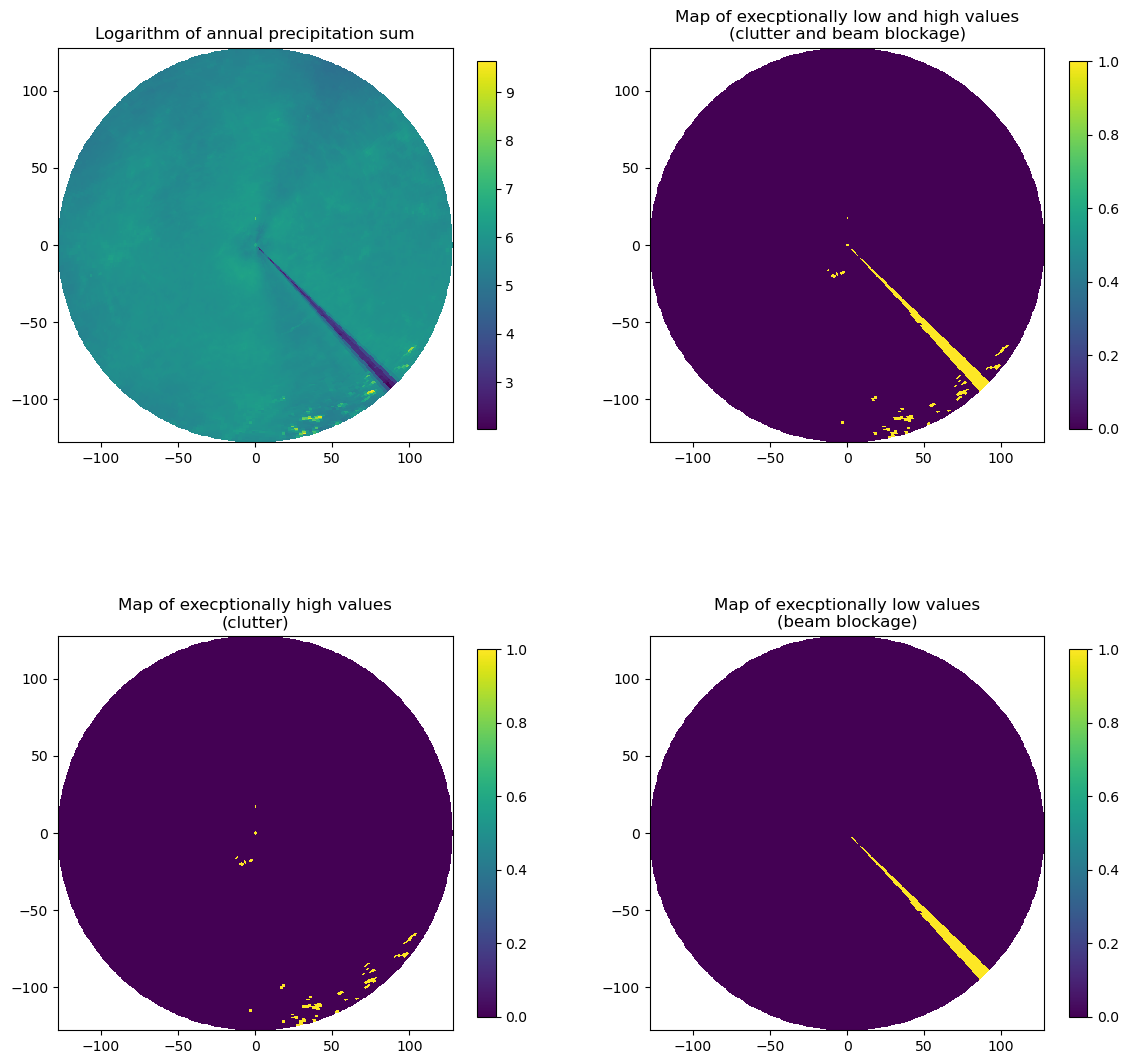
Plot results#
[4]:
fig = pl.figure(figsize=(14, 14))
ax = fig.add_subplot(221)
ax, pm = plot_ppi(np.log(yearsum), ax=ax)
pl.title("Logarithm of annual precipitation sum")
pl.colorbar(pm, shrink=0.75)
ax = fig.add_subplot(222)
ax, pm = plot_ppi(mask.astype(bool), ax=ax)
pl.title("Map of execptionally low and high values\n(clutter and beam blockage)")
pl.colorbar(pm, shrink=0.75)
ax = fig.add_subplot(223)
ax, pm = plot_ppi(mask == 1, ax=ax)
pl.title("Map of execptionally high values\n(clutter)")
pl.colorbar(pm, shrink=0.75)
ax = fig.add_subplot(224)
ax, pm = plot_ppi(mask == 2, ax=ax)
pl.title("Map of execptionally low values\n(beam blockage)")
pl.colorbar(pm, shrink=0.75)
[4]:
<matplotlib.colorbar.Colorbar at 0x7f47e5bddd50>