xarray CfRadial2 backend
In this example, we read CfRadial2 data files using the xarray cfradial2 backend.
[1]:
import wradlib as wrl
import warnings

warnings.filterwarnings("ignore")
import matplotlib.pyplot as pl
import numpy as np
import xarray as xr

try:
    get_ipython().run_line_magic("matplotlib inline")
except:
    pl.ion()
/home/runner/micromamba-root/envs/wradlib-notebooks/lib/python3.11/site-packages/tqdm/auto.py:22: TqdmWarning: IProgress not found. Please update jupyter and ipywidgets. See https://ipywidgets.readthedocs.io/en/stable/user_install.html
  from .autonotebook import tqdm as notebook_tqdm
Load CfRadial2 Volume Data
[2]:
fpath = "netcdf/cfrad.20080604_002217_000_SPOL_v36_SUR_cfradial2.nc"
f = wrl.util.get_wradlib_data_file(fpath)
vol = wrl.io.open_cfradial2_dataset(f)
Downloading file 'netcdf/cfrad.20080604_002217_000_SPOL_v36_SUR_cfradial2.nc' from 'https://github.com/wradlib/wradlib-data/raw/pooch/data/netcdf/cfrad.20080604_002217_000_SPOL_v36_SUR_cfradial2.nc' to '/home/runner/work/wradlib-notebooks/wradlib-notebooks/wradlib-data'.
Inspect RadarVolume
[3]:
display(vol)
<wradlib.RadarVolume>
Dimension(s): (sweep: 9)
Elevation(s): (0.5, 1.1, 1.8, 2.6, 3.6, 4.7, 6.5, 9.1, 12.8)
Inspect root group
The sweep dimension contains the number of scans in this radar volume. Further the dataset consists of variables (location coordinates, time_coverage) and attributes (Conventions, metadata).
[4]:
vol.root
[4]:
<xarray.Dataset>
Dimensions:              (sweep: 9)
Dimensions without coordinates: sweep
Data variables:
    volume_number        int64 0
    platform_type        <U5 'fixed'
    instrument_type      <U5 'radar'
    primary_axis         <U6 'axis_z'
    time_coverage_start  <U20 '2008-06-04T00:15:03Z'
    time_coverage_end    <U20 '2008-06-04 00:22:16Z'
    latitude             float64 ...
    longitude            float64 ...
    altitude             float64 ...
    sweep_group_name     (sweep) <U7 'sweep_0' 'sweep_1' ... 'sweep_7' 'sweep_8'
    sweep_fixed_angle    (sweep) float32 0.4999 1.099 1.802 ... 6.498 9.102 12.8
Attributes:
    version:          None
    title:            None
    institution:      None
    references:       None
    source:           None
    history:          None
    comment:          im/exported using wradlib
    instrument_name:  None
fixed_angle: 0.5Inspect sweep group(s)
The sweep-groups can be accessed via their respective keys. The dimensions consist of range and time with added coordinates azimuth, elevation, range and time. There will be variables like radar moments (DBZH etc.) and sweep-dependend metadata (like fixed_angle, sweep_mode etc.).
[5]:
display(vol[0])
<xarray.Dataset>
Dimensions:             (azimuth: 480, range: 996)
Coordinates:
    sweep_mode          <U20 ...
    rtime               (azimuth) datetime64[ns] 2008-06-04T00:15:34 ... 2008...
  * range               (range) float32 150.0 300.0 ... 1.492e+05 1.494e+05
  * azimuth             (azimuth) float32 0.0 0.75 1.5 ... 357.8 358.5 359.2
    elevation           (azimuth) float32 ...
    longitude           float64 ...
    latitude            float64 ...
    altitude            float64 ...
    time                datetime64[ns] 2008-06-04T00:15:03
Data variables: (12/16)
    sweep_number        int32 ...
    polarization_mode   |S32 ...
    prt_mode            |S32 ...
    follow_mode         |S32 ...
    sweep_fixed_angle   float32 0.4999
    target_scan_rate    float32 ...
    ...                  ...
    antenna_transition  (azimuth) int8 ...
    n_samples           (azimuth) int32 ...
    r_calib_index       (azimuth) int8 ...
    scan_rate           (azimuth) float32 ...
    DBZ                 (azimuth, range) float32 ...
    VR                  (azimuth, range) float32 ...
Attributes:
fixed_angle: 0.5Goereferencing
[6]:
swp = vol[0].copy().pipe(wrl.georef.georeference_dataset)
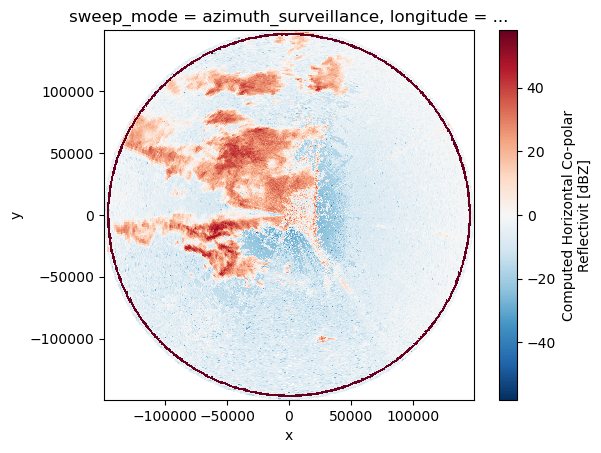
Plotting
[7]:
swp.DBZ.plot.pcolormesh(x="x", y="y")
pl.gca().set_aspect("equal")
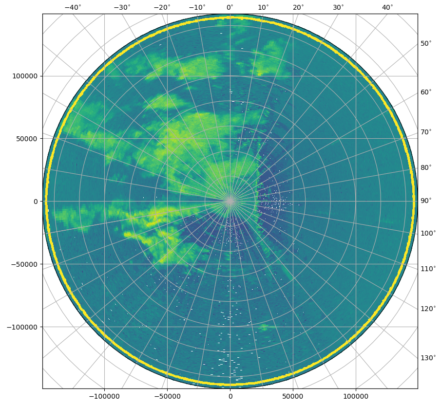
[8]:
fig = pl.figure(figsize=(10, 10))
swp.DBZ.wradlib.plot_ppi(proj="cg", fig=fig)
[8]:
<matplotlib.collections.QuadMesh at 0x7f588b0fdc10>
[9]:
import cartopy
import cartopy.crs as ccrs
import cartopy.feature as cfeature

map_trans = ccrs.AzimuthalEquidistant(
    central_latitude=swp.latitude.values, central_longitude=swp.longitude.values
)
[10]:
map_proj = ccrs.AzimuthalEquidistant(
    central_latitude=swp.latitude.values, central_longitude=swp.longitude.values
)
pm = swp.DBZ.wradlib.plot_ppi(proj=map_proj)
ax = pl.gca()
ax.gridlines(crs=map_proj)
print(ax)
< GeoAxes: +proj=aeqd +ellps=WGS84 +lon_0=120.43350219726562 +lat_0=22.52669906616211 +x_0=0.0 +y_0=0.0 +no_defs +type=crs >
[11]:
map_proj = ccrs.Mercator(central_longitude=swp.longitude.values)
fig = pl.figure(figsize=(10, 8))
ax = fig.add_subplot(111, projection=map_proj)
pm = swp.DBZ.wradlib.plot_ppi(ax=ax)
ax.gridlines(draw_labels=True)
[11]:
<cartopy.mpl.gridliner.Gridliner at 0x7f588b0fba10>
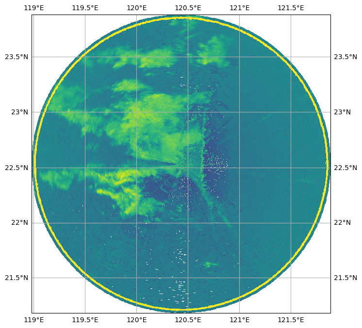
[12]:
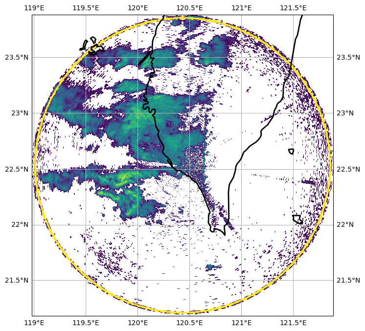
import cartopy.feature as cfeature


def plot_borders(ax):
    borders = cfeature.NaturalEarthFeature(
        category="physical", name="coastline", scale="10m", facecolor="none"
    )
    ax.add_feature(borders, edgecolor="black", lw=2, zorder=4)


map_proj = ccrs.Mercator(central_longitude=swp.longitude.values)
fig = pl.figure(figsize=(10, 8))
ax = fig.add_subplot(111, projection=map_proj)

DBZ = swp.DBZ
pm = DBZ.where(DBZ > 0).wradlib.plot_ppi(ax=ax)
plot_borders(ax)
ax.gridlines(draw_labels=True)
[12]:
<cartopy.mpl.gridliner.Gridliner at 0x7f587bd38750>
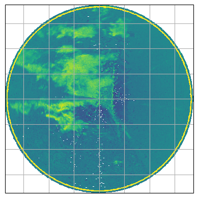
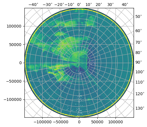
[13]:
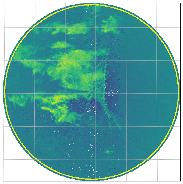
import matplotlib.path as mpath

theta = np.linspace(0, 2 * np.pi, 100)
center, radius = [0.5, 0.5], 0.5
verts = np.vstack([np.sin(theta), np.cos(theta)]).T
circle = mpath.Path(verts * radius + center)

map_proj = ccrs.AzimuthalEquidistant(
    central_latitude=swp.latitude.values,
    central_longitude=swp.longitude.values,
)
fig = pl.figure(figsize=(10, 8))
ax = fig.add_subplot(111, projection=map_proj)
ax.set_boundary(circle, transform=ax.transAxes)

pm = swp.DBZ.wradlib.plot_ppi(proj=map_proj, ax=ax)
ax = pl.gca()
ax.gridlines(crs=map_proj)
[13]:
<cartopy.mpl.gridliner.Gridliner at 0x7f588bc92350>

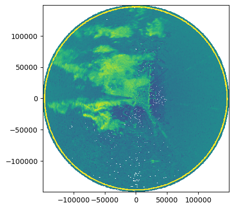
[14]:
fig = pl.figure(figsize=(10, 8))
proj = ccrs.AzimuthalEquidistant(
    central_latitude=swp.latitude.values, central_longitude=swp.longitude.values
)
ax = fig.add_subplot(111, projection=proj)
pm = swp.DBZ.wradlib.plot_ppi(ax=ax)
ax.gridlines()
[14]:
<cartopy.mpl.gridliner.Gridliner at 0x7f587bb22490>
[15]:
swp.DBZ.wradlib.plot_ppi()
[15]:
<matplotlib.collections.QuadMesh at 0x7f587bdc2ed0>
Inspect radar moments
The DataArrays can be accessed by key or by attribute. Each DataArray has dimensions and coordinates of it’s parent dataset. There are attributes connected which are defined by Cf/Radial standard.
[16]:
display(swp.DBZ)
<xarray.DataArray 'DBZ' (azimuth: 480, range: 996)>
array([[ 20.699957, 39.96934 , 29.650644, ..., -2.799595, -3.549335,
-1.650112],
[ 13.829709, 35.710747, 8.869345, ..., -18.780428, -3.080303,
-4.519378],
[ -9.129745, 14.810412, 4.539685, ..., 0.179822, -0.550375,
-3.519132],
...,
[ 5.889927, 26.049406, 32.379555, ..., -2.550866, -1.060269,
-1.900617],
[ 0.959765, 23.579884, 9.29929 , ..., -8.680257, -5.039932,
-2.410512],
[ 20.079912, 39.15031 , 13.190121, ..., -4.91912 , -3.160252,
-1.319658]], dtype=float32)
Coordinates: (12/15)
sweep_mode <U20 'azimuth_surveillance'
rtime (azimuth) datetime64[ns] 2008-06-04T00:15:34 ... 2008-06-04T0...
* range (range) float32 150.0 300.0 450.0 ... 1.492e+05 1.494e+05
* azimuth (azimuth) float32 0.0 0.75 1.5 2.25 ... 357.0 357.8 358.5 359.2
elevation (azimuth) float32 0.5164 0.5219 0.5164 ... 0.5219 0.5219 0.5219
longitude float64 120.4
... ...
x (azimuth, range) float32 -6.556e-06 -1.311e-05 ... -1.955e+03
y (azimuth, range) float32 150.0 300.0 ... 1.492e+05 1.493e+05
z (azimuth, range) float32 46.0 47.0 48.0 ... 2.714e+03 2.718e+03
gr (azimuth, range) float32 150.0 300.0 ... 1.492e+05 1.494e+05
rays (azimuth, range) float32 0.0 0.0 0.0 0.0 ... 359.2 359.2 359.2
bins (azimuth, range) float32 150.0 300.0 ... 1.492e+05 1.494e+05
Attributes:
long_name: Computed Horizontal Co-polar Reflectivit
standard_name: equivalent_reflectivity_factor
units: dBZ
threshold_field_name:
threshold_value: -9999.0
sampling_ratio: 1.0
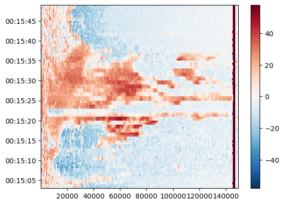
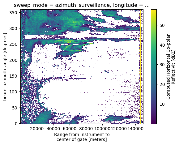
grid_mapping: grid_mappingCreate simple plot
Using xarray features a simple plot can be created like this. Note the sortby('time') method, which sorts the radials by time.
[17]:
swp.DBZ.sortby("rtime").plot(x="range", y="rtime", add_labels=False)
[17]:
<matplotlib.collections.QuadMesh at 0x7f587bc1ecd0>
[18]:
fig = pl.figure(figsize=(5, 5))
pm = swp.DBZ.wradlib.plot_ppi(proj={"latmin": 33e3}, fig=fig)
Mask some values
[19]:
swp["DBZ"] = swp["DBZ"].where(swp["DBZ"] >= 0)
swp["DBZ"].plot()
[19]:
<matplotlib.collections.QuadMesh at 0x7f587bfa5850>
Export to ODIM and CfRadial2
[20]:
vol.to_odim("cfradial2_as_odim.h5")
vol.to_cfradial2("cfradial2_as_cfradial2.nc")
Import again
[21]:
vola = wrl.io.open_odim_dataset(
    "cfradial2_as_odim.h5",
    decode_coords=True,
    backend_kwargs=dict(keep_azimuth=True, keep_elevation=True, reindex_angle=False),
)
[22]:
volb = wrl.io.open_cfradial2_dataset("cfradial2_as_cfradial2.nc")
Check equality
Some variables need to be dropped, since they are not exported to the other standards or differ slightly (eg. re-indexed ray times).
[23]:
drop = set(vol[0]) ^ set(vola[0]) | set({"rtime"})
xr.testing.assert_allclose(vol.root, vola.root)
xr.testing.assert_allclose(
    vol[0].drop_vars(drop), vola[0].drop_vars(drop, errors="ignore")
)
xr.testing.assert_allclose(vol.root, volb.root)
xr.testing.assert_equal(vol[0], volb[0])
xr.testing.assert_allclose(vola.root, volb.root)
xr.testing.assert_allclose(
    vola[0].drop_vars(drop, errors="ignore"), volb[0].drop_vars(drop, errors="ignore")
)