xarray CfRadial1 backend
In this example, we read and write CfRadial1 data files using the xarray wradlib-cfradial1 backend.
[1]:
import wradlib as wrl
import warnings

warnings.filterwarnings("ignore")
import matplotlib.pyplot as pl
import numpy as np
import xarray as xr

try:
    get_ipython().run_line_magic("matplotlib inline")
except:
    pl.ion()
/home/runner/micromamba-root/envs/wradlib-notebooks/lib/python3.11/site-packages/tqdm/auto.py:22: TqdmWarning: IProgress not found. Please update jupyter and ipywidgets. See https://ipywidgets.readthedocs.io/en/stable/user_install.html
  from .autonotebook import tqdm as notebook_tqdm
Load CfRadial1 Volume Data
[2]:
fpath = "netcdf/cfrad.20080604_002217_000_SPOL_v36_SUR.nc"
f = wrl.util.get_wradlib_data_file(fpath)
vol = wrl.io.open_cfradial1_dataset(f)
Downloading file 'netcdf/cfrad.20080604_002217_000_SPOL_v36_SUR.nc' from 'https://github.com/wradlib/wradlib-data/raw/pooch/data/netcdf/cfrad.20080604_002217_000_SPOL_v36_SUR.nc' to '/home/runner/work/wradlib-notebooks/wradlib-notebooks/wradlib-data'.
Inspect RadarVolume
[3]:
display(vol)
<wradlib.RadarVolume>
Dimension(s): (sweep: 9)
Elevation(s): (0.5, 1.1, 1.8, 2.6, 3.6, 4.7, 6.5, 9.1, 12.8)
Inspect root group
The sweep dimension contains the number of scans in this radar volume. Further the dataset consists of variables (location coordinates, time_coverage) and attributes (Conventions, metadata).
[4]:
vol.root
[4]:
<xarray.Dataset>
Dimensions:              (sweep: 9)
Dimensions without coordinates: sweep
Data variables:
    volume_number        int64 0
    platform_type        <U5 'fixed'
    instrument_type      <U5 'radar'
    primary_axis         <U6 'axis_z'
    time_coverage_start  <U20 '2008-06-04T00:15:03Z'
    time_coverage_end    <U20 '2008-06-04 00:22:17Z'
    latitude             float64 ...
    longitude            float64 ...
    altitude             float64 ...
    sweep_group_name     (sweep) <U7 'sweep_0' 'sweep_1' ... 'sweep_7' 'sweep_8'
    sweep_fixed_angle    (sweep) float32 0.4999 1.099 1.802 ... 6.498 9.102 12.8
Attributes:
    version:          None
    title:            None
    institution:      None
    references:       None
    source:           None
    history:          None
    comment:          im/exported using wradlib
instrument_name: NoneInspect sweep group(s)
The sweep-groups can be accessed via their respective keys. The dimensions consist of range and time with added coordinates azimuth, elevation, range and time. There will be variables like radar moments (DBZH etc.) and sweep-dependend metadata (like fixed_angle, sweep_mode etc.).
[5]:
display(vol[0])
<xarray.Dataset>
Dimensions:                    (azimuth: 483, range: 996)
Coordinates:
    sweep_mode                 <U20 'azimuth_surveillance'
    rtime                      (azimuth) datetime64[ns] 2008-06-04T00:15:34 ....
  * range                      (range) float32 150.0 300.0 ... 1.494e+05
  * azimuth                    (azimuth) float32 0.0 0.75 1.5 ... 358.5 359.2
    elevation                  (azimuth) float32 ...
    latitude                   float64 ...
    longitude                  float64 ...
    altitude                   float64 ...
    time                       datetime64[ns] 2008-06-04T00:15:03
Data variables: (12/17)
    sweep_number               int32 ...
    prt_mode                   |S32 ...
    follow_mode                |S32 ...
    sweep_fixed_angle          float32 0.4999
    pulse_width                (azimuth) timedelta64[ns] ...
    prt                        (azimuth) timedelta64[ns] ...
    ...                         ...
    r_calib_index              (azimuth) int8 ...
    measured_transmit_power_h  (azimuth) float32 ...
    measured_transmit_power_v  (azimuth) float32 ...
    scan_rate                  (azimuth) float32 ...
    DBZ                        (azimuth, range) float32 ...
VR (azimuth, range) float32 ...Georeferencing
[6]:
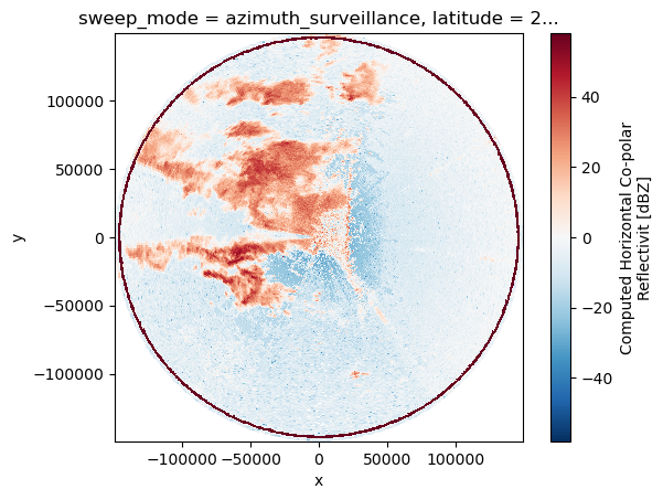
swp = vol[0].copy().pipe(wrl.georef.georeference_dataset)
Plotting
[7]:
swp.DBZ.plot.pcolormesh(x="x", y="y")
pl.gca().set_aspect("equal")
[8]:
fig = pl.figure(figsize=(10, 10))
swp.DBZ.wradlib.plot_ppi(proj="cg", fig=fig)
[8]:
<matplotlib.collections.QuadMesh at 0x7f1f84767ed0>
[9]:
import cartopy
import cartopy.crs as ccrs
import cartopy.feature as cfeature

map_trans = ccrs.AzimuthalEquidistant(
    central_latitude=swp.latitude.values, central_longitude=swp.longitude.values
)
[10]:
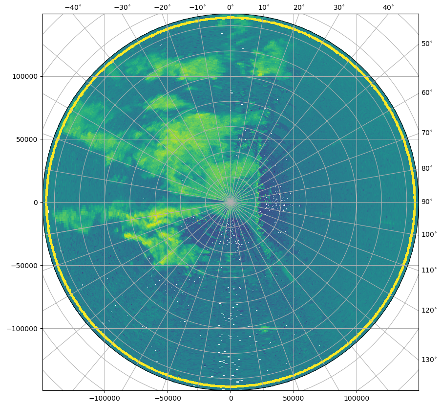
map_proj = ccrs.AzimuthalEquidistant(
    central_latitude=swp.latitude.values, central_longitude=swp.longitude.values
)
pm = swp.DBZ.wradlib.plot_ppi(proj=map_proj)
ax = pl.gca()
ax.gridlines(crs=map_proj)
print(ax)
< GeoAxes: +proj=aeqd +ellps=WGS84 +lon_0=120.43350219726562 +lat_0=22.52669906616211 +x_0=0.0 +y_0=0.0 +no_defs +type=crs >
[11]:
map_proj = ccrs.Mercator(central_longitude=swp.longitude.values)
fig = pl.figure(figsize=(10, 8))
ax = fig.add_subplot(111, projection=map_proj)
pm = swp.DBZ.wradlib.plot_ppi(ax=ax)
ax.gridlines(draw_labels=True)
[11]:
<cartopy.mpl.gridliner.Gridliner at 0x7f1f8ffe9290>
[12]:
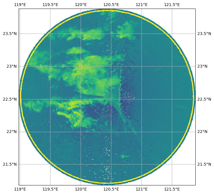
import cartopy.feature as cfeature
def plot_borders(ax):
borders = cfeature.NaturalEarthFeature(
category="physical", name="coastline", scale="10m", facecolor="none"
)
ax.add_feature(borders, edgecolor="black", lw=2, zorder=4)
map_proj = ccrs.Mercator(central_longitude=swp.longitude.values)
fig = pl.figure(figsize=(10, 8))
ax = fig.add_subplot(111, projection=map_proj)
DBZ = swp.DBZ
pm = DBZ.where(DBZ > 0).wradlib.plot_ppi(ax=ax)
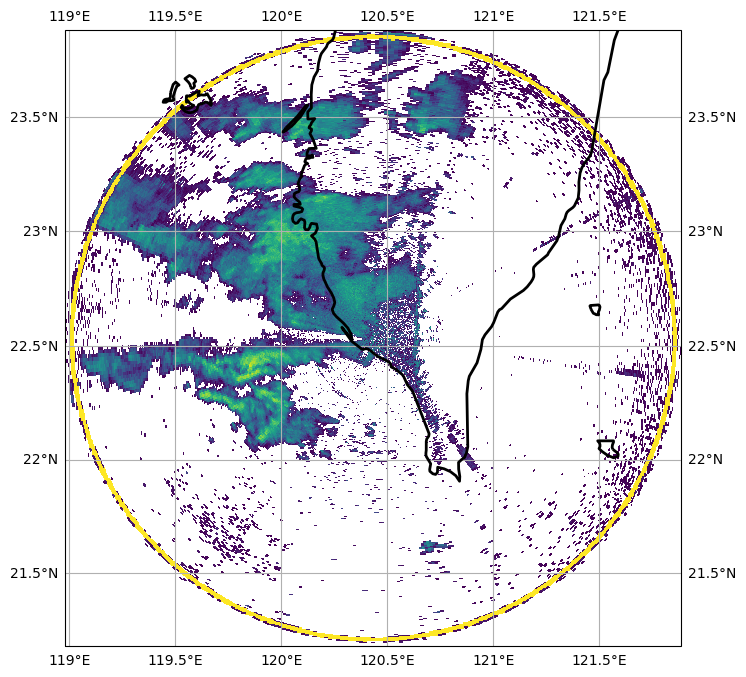
plot_borders(ax)
ax.gridlines(draw_labels=True)
[12]:
<cartopy.mpl.gridliner.Gridliner at 0x7f1f847d8a90>
[13]:
import matplotlib.path as mpath
theta = np.linspace(0, 2 * np.pi, 100)
center, radius = [0.5, 0.5], 0.5
verts = np.vstack([np.sin(theta), np.cos(theta)]).T
circle = mpath.Path(verts * radius + center)
map_proj = ccrs.AzimuthalEquidistant(
central_latitude=swp.latitude.values,
central_longitude=swp.longitude.values,
)
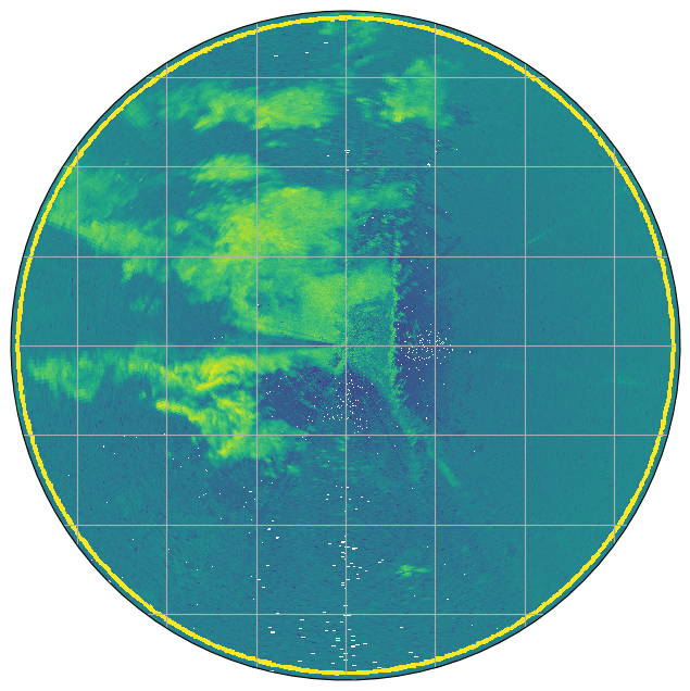
fig = pl.figure(figsize=(10, 8))
ax = fig.add_subplot(111, projection=map_proj)
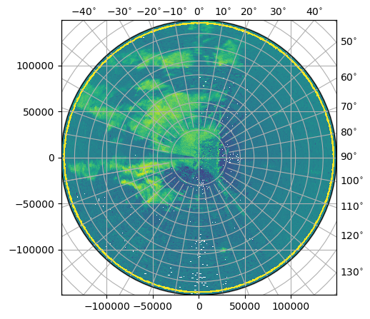
ax.set_boundary(circle, transform=ax.transAxes)
pm = swp.DBZ.wradlib.plot_ppi(proj=map_proj, ax=ax)
ax = pl.gca()
ax.gridlines(crs=map_proj)
[13]:
<cartopy.mpl.gridliner.Gridliner at 0x7f1f9124ee90>
[14]:
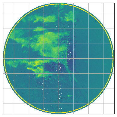
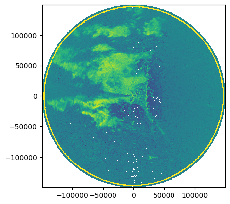
fig = pl.figure(figsize=(10, 8))
proj = ccrs.AzimuthalEquidistant(
    central_latitude=swp.latitude.values, central_longitude=swp.longitude.values
)
ax = fig.add_subplot(111, projection=proj)
pm = swp.DBZ.wradlib.plot_ppi(ax=ax)
ax.gridlines()
[14]:
<cartopy.mpl.gridliner.Gridliner at 0x7f1f8d9748d0>

[15]:
swp.DBZ.wradlib.plot_ppi()
[15]:
<matplotlib.collections.QuadMesh at 0x7f1f8d917a10>
Inspect radar moments
The DataArrays can be accessed by key or by attribute. Each DataArray has dimensions and coordinates of it’s parent dataset. There are attributes connected which are defined by Cf/Radial standard.
[16]:
display(swp.DBZ)
<xarray.DataArray 'DBZ' (azimuth: 483, range: 996)>
array([[ 20.699957,  39.96934 ,  29.650644, ...,  -2.799595,  -3.549335,
         -1.650112],
       [ 13.829709,  35.710747,   8.869345, ..., -18.780428,  -3.080303,
         -4.519378],
       [ -9.129745,  14.810412,   4.539685, ...,   0.179822,  -0.550375,
         -3.519132],
       ...,
       [  5.889927,  26.049406,  32.379555, ...,  -2.550866,  -1.060269,
         -1.900617],
       [  0.959765,  23.579884,   9.29929 , ...,  -8.680257,  -5.039932,
         -2.410512],
       [ 20.079912,  39.15031 ,  13.190121, ...,  -4.91912 ,  -3.160252,
         -1.319658]], dtype=float32)
Coordinates: (12/15)
    sweep_mode  <U20 'azimuth_surveillance'
    rtime       (azimuth) datetime64[ns] 2008-06-04T00:15:34 ... 2008-06-04T0...
  * range       (range) float32 150.0 300.0 450.0 ... 1.492e+05 1.494e+05
  * azimuth     (azimuth) float32 0.0 0.75 1.5 2.25 ... 357.0 357.8 358.5 359.2
    elevation   (azimuth) float32 0.5164 0.5219 0.5164 ... 0.5219 0.5219 0.5219
    latitude    float64 22.53
    ...          ...
    x           (azimuth, range) float32 -6.556e-06 -1.311e-05 ... -1.955e+03
    y           (azimuth, range) float32 150.0 300.0 ... 1.492e+05 1.493e+05
    z           (azimuth, range) float32 46.0 47.0 48.0 ... 2.714e+03 2.718e+03
    gr          (azimuth, range) float32 150.5 300.5 ... 1.492e+05 1.494e+05
    rays        (azimuth, range) float32 0.0 0.0 0.0 0.0 ... 359.2 359.2 359.2
    bins        (azimuth, range) float32 150.0 300.0 ... 1.492e+05 1.494e+05
Attributes:
    long_name:             Computed Horizontal Co-polar Reflectivit
    standard_name:         equivalent_reflectivity_factor
    units:                 dBZ
    threshold_field_name:
    threshold_value:       -9999.0
    sampling_ratio:        1.0
grid_mapping: grid_mappingCreate simple plot
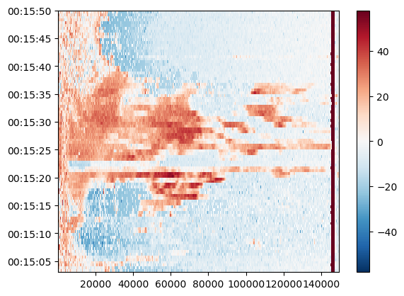
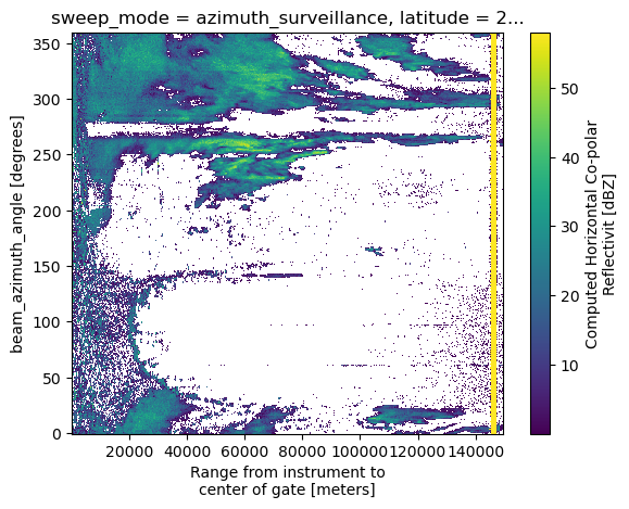
Using xarray features a simple plot can be created like this. Note the sortby('time') method, which sorts the radials by time.
[17]:
swp.DBZ.sortby("rtime").plot(x="range", y="rtime", add_labels=False)
[17]:
<matplotlib.collections.QuadMesh at 0x7f1f8464a4d0>
[18]:
fig = pl.figure(figsize=(5, 5))
pm = swp.DBZ.wradlib.plot_ppi(proj={"latmin": 33e3}, fig=fig)
Mask some values
[19]:
swp["DBZ"] = swp["DBZ"].where(swp["DBZ"] >= 0)
swp["DBZ"].plot()
[19]:
<matplotlib.collections.QuadMesh at 0x7f1f8d909190>
Export to ODIM and CfRadial2
[20]:
vol.to_odim("cfradial1_as_odim.h5")
vol.to_cfradial2("cfradial1_as_cfradial2.nc")
Import again
[21]:
vola = wrl.io.open_odim_dataset(
    "cfradial1_as_odim.h5",
    decode_coords=True,
    backend_kwargs=dict(keep_azimuth=True, keep_elevation=True, reindex_angle=False),
)
[22]:
volb = wrl.io.open_cfradial2_dataset("cfradial1_as_cfradial2.nc")
Check equality
Some variables need to be dropped, since they are not exported to the other standards.
[23]:
drop = set(vol[0]) ^ set(vola[0]) | set({"rtime"})
print(drop)
xr.testing.assert_allclose(vol.root, vola.root)
xr.testing.assert_allclose(
    vol[0].drop_vars(drop), vola[0].drop_vars(drop, errors="ignore")
)

xr.testing.assert_allclose(vol.root, volb.root)
xr.testing.assert_equal(vol[0], volb[0])

xr.testing.assert_allclose(vola.root, volb.root)
xr.testing.assert_allclose(
    vola[0].drop_vars(drop, errors="ignore"), volb[0].drop_vars(drop, errors="ignore")
)
{'pulse_width', 'nyquist_velocity', 'unambiguous_range', 'scan_rate', 'measured_transmit_power_h', 'measured_transmit_power_v', 'n_samples', 'prt', 'prt_ratio', 'rtime', 'antenna_transition', 'r_calib_index'}
More CfRadial1 loading mechanisms
Use xr.open_dataset to retrieve explicit group
Warning
Since \(\omega radlib\) version 1.18 the xarray backend engines for polar radar data have been renamed and prepended with wradlib- (eg. cfradial1 -> wradlib-cfradial1). This was necessary to avoid clashes with the new xradar-package, which will eventually replace the wradlib engines. Users have to make sure to check which engine to use for their use-case when using xarray.open_dataset. Users might install and test xradar, and
check if it is already robust enough for their use-cases (by using xradar’s engine="cfradial1".
Since \(\omega radlib\) version 1.19 the xarray backend engines for polar radar data have been deprecated. The functionality is kept until wradlib version 2.0, when the backend-code will be removed completely. wradlib is importing that functionality from xradar-package whenever and wherever necessary.
Below we use a compatibility layer in wradlib to give users the chance to adapt their code. The first minimal change is that for every backend the group-layout is conforming to the CfRadial-standard naming scheme (sweep_0, sweep_1, etc.).
Below you can inspect the main differences of the wradlib compatibility layer and the plain xradar implementation.
use wradlib compatibility layer
[24]:
swp_a = xr.open_dataset(
    f,
    engine="wradlib-cfradial1",
    group="sweep_1",
    backend_kwargs=dict(reindex_angle=False),
)
display(swp_a)
<xarray.Dataset>
Dimensions:                    (azimuth: 483, range: 996)
Coordinates:
    sweep_mode                 |S32 ...
    rtime                      (azimuth) datetime64[ns] ...
  * range                      (range) float32 150.0 300.0 ... 1.494e+05
  * azimuth                    (azimuth) float32 0.0 0.75 1.5 ... 358.5 359.2
    elevation                  (azimuth) float32 ...
    latitude                   float64 ...
    longitude                  float64 ...
    altitude                   float64 ...
    time                       datetime64[ns] ...
Data variables: (12/17)
    sweep_number               int32 ...
    prt_mode                   |S32 ...
    follow_mode                |S32 ...
    sweep_fixed_angle          float32 ...
    pulse_width                (azimuth) timedelta64[ns] ...
    prt                        (azimuth) timedelta64[ns] ...
    ...                         ...
    r_calib_index              (azimuth) int8 ...
    measured_transmit_power_h  (azimuth) float32 ...
    measured_transmit_power_v  (azimuth) float32 ...
    scan_rate                  (azimuth) float32 ...
    DBZ                        (azimuth, range) float32 ...
    VR                         (azimuth, range) float32 ...
Attributes:
fixed_angle: 1.0986use xradar backend
[25]:
swp_b = xr.open_dataset(
    f, engine="cfradial1", group="sweep_1", backend_kwargs=dict(reindex_angle=False)
)
display(swp_b)
<xarray.Dataset>
Dimensions:                    (azimuth: 483, range: 996)
Coordinates:
    time                       (azimuth) datetime64[ns] ...
  * range                      (range) float32 150.0 300.0 ... 1.494e+05
  * azimuth                    (azimuth) float32 0.0 0.75 1.5 ... 358.5 359.2
    elevation                  (azimuth) float32 ...
    latitude                   float64 ...
    longitude                  float64 ...
    altitude                   float64 ...
Data variables: (12/18)
    sweep_number               int32 ...
    sweep_mode                 |S32 ...
    prt_mode                   |S32 ...
    follow_mode                |S32 ...
    sweep_fixed_angle          float32 ...
    pulse_width                (azimuth) timedelta64[ns] ...
    ...                         ...
    r_calib_index              (azimuth) int8 ...
    measured_transmit_power_h  (azimuth) float32 ...
    measured_transmit_power_v  (azimuth) float32 ...
    scan_rate                  (azimuth) float32 ...
    DBZ                        (azimuth, range) float32 ...
    VR                         (azimuth, range) float32 ...