Intro#
This chapter shows simple loading and visualization of RADOLAN data.
import warnings

warnings.filterwarnings("ignore")

import matplotlib.pyplot as plt
import numpy as np
import wradlib as wrl
import xarray as xr
wradlib reader#
All RADOLAN composite products can be read by wradlib.io.read_radolan_composite():
data, metadata = wradlib.io.read_radolan_composite("mydrive:/path/to/my/file/filename")
Here, data is a two dimensional integer or float array of shape (number of rows, number of columns). metadata is a dictionary which provides metadata from the files header section, e.g. using the keys producttype, datetime, intervalseconds, nodataflag.
Import data#
# load radolan files
rw_filename = "../data/misc/raa01-rw_10000-1408102050-dwd---bin.gz"
rwdata, rwattrs = wrl.io.read_radolan_composite(rw_filename)
# print the available attributes
print("RW Attributes:", rwattrs)
RW Attributes: {'producttype': 'RW', 'datetime': datetime.datetime(2014, 8, 10, 20, 50), 'radarid': '10000', 'nrow': 900, 'ncol': 900, 'datasize': 1620000, 'formatversion': 3, 'maxrange': '150 km', 'radolanversion': '2.13.1', 'precision': 0.1, 'intervalseconds': 3600, 'radarlocations': ['boo', 'ros', 'emd', 'hnr', 'umd', 'pro', 'ess', 'asd', 'neu', 'nhb', 'oft', 'tur', 'isn', 'fbg', 'mem'], 'nodataflag': -9999, 'secondary': array([   799,    800,    801, ..., 806263, 806264, 807163],
      shape=(23032,)), 'nodatamask': array([     0,      1,      2, ..., 809997, 809998, 809999],
      shape=(179061,)), 'cluttermask': array([], dtype=int64)}
Mask and get coordinates#
The Grid - Sphere coordinates can be calculated with wradlib.georef.get_radolan_grid().
# do some masking
sec = rwattrs["secondary"]
rwdata.flat[sec] = -9999
rwdata = np.ma.masked_equal(rwdata, -9999)
# Get coordinates
radolan_grid_xy = wrl.georef.get_radolan_grid(900, 900)
x = radolan_grid_xy[:, :, 0]
y = radolan_grid_xy[:, :, 1]
Simple wradlib plot#
With the following code snippet the RW-product is visualized in the Polar Stereographic Projection. For more details, refer to matplotlib.pyplot.pcolormesh().
# plot function
plt.pcolormesh(x, y, rwdata, cmap="viridis")
cb = plt.colorbar(shrink=0.75)
cb.set_label("mm * h-1")
plt.title("RADOLAN RW Product Polar Stereo \n" + rwattrs["datetime"].isoformat())
plt.grid(color="r")
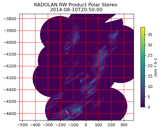
Data: RADOLAN — Deutscher Wetterdienst (DWD). Licensed under CC BY 4.0.
A much more comprehensive section using several RADOLAN composites is shown in chapter Legacy and ODIM_H5.
Xarray backend#
RADOLAN binary format data will be imported into an xarray.Dataset with attached coordinates.
# load radolan files
rw_filename = "../data/misc/raa01-rw_10000-1408102050-dwd---bin.gz"
ds = wrl.io.open_radolan_dataset(rw_filename)
# print the xarray dataset
display(ds)
<xarray.Dataset> Size: 3MB
Dimensions:  (y: 900, x: 900, time: 1)
Coordinates:
  * y        (y) float64 7kB -4.658e+06 -4.657e+06 ... -3.76e+06 -3.759e+06
  * x        (x) float64 7kB -5.23e+05 -5.22e+05 -5.21e+05 ... 3.75e+05 3.76e+05
  * time     (time) datetime64[ns] 8B 2014-08-10T20:50:00
Data variables:
    RW       (y, x) float32 3MB ...
    crs      int64 8B ...
Attributes:
    radarid:         10000
    formatversion:   3
    radolanversion:  2.13.1
radarlocations: ['boo', 'ros', 'emd', 'hnr', 'umd', 'pro', 'ess', 'asd',...Simple xarray plot#
ds.RW.plot()
<matplotlib.collections.QuadMesh at 0x7619f16d8550>
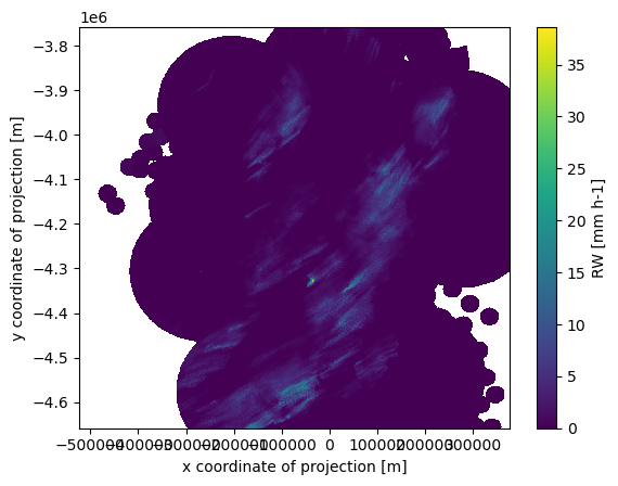
Data: RADOLAN — Deutscher Wetterdienst (DWD). Licensed under CC BY 4.0.
Simple selection#
ds.RW.sel(x=slice(-100000, 100000), y=slice(-4400000, -4200000)).plot()
<matplotlib.collections.QuadMesh at 0x7619f15e4e10>
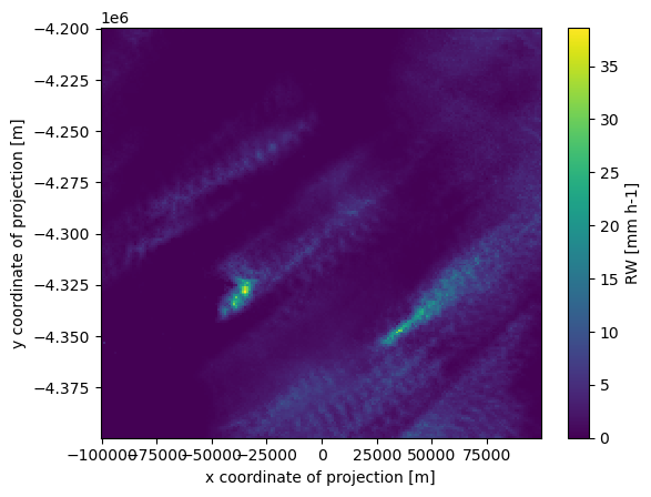
Data: RADOLAN — Deutscher Wetterdienst (DWD). Licensed under CC BY 4.0.
Map plot using cartopy#
We will use cartopy.crs.Stereographic for map-making.
import cartopy.crs as ccrs

map_proj = ccrs.Stereographic(
    true_scale_latitude=60.0, central_latitude=90.0, central_longitude=10.0
)
fig = plt.figure(figsize=(10, 8))
ds.RW.plot(subplot_kws=dict(projection=map_proj))
ax = plt.gca()
ax.gridlines(draw_labels=True, y_inline=False)
<cartopy.mpl.gridliner.Gridliner at 0x7619f14fcec0>
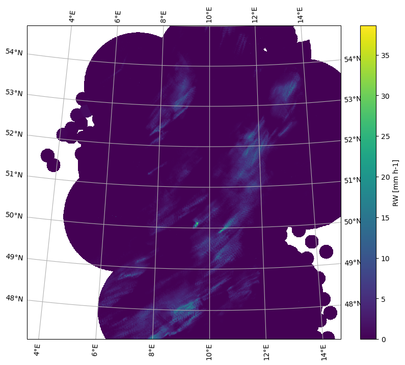
Data: RADOLAN — Deutscher Wetterdienst (DWD). Licensed under CC BY 4.0.
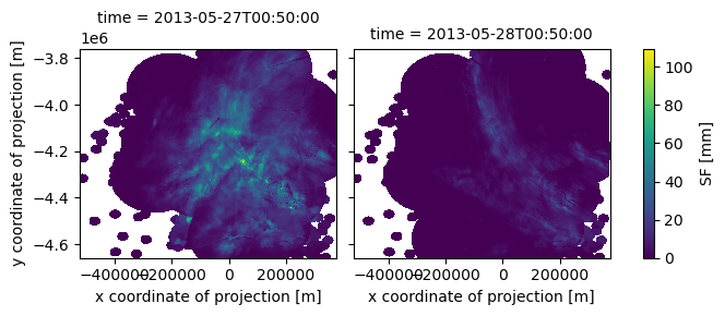
Open multiple files#
# load radolan files
sf_filenames = [
    "../data/misc/raa01-sf_10000-1305270050-dwd---bin.gz",
    "../data/misc/raa01-sf_10000-1305280050-dwd---bin.gz",
]
ds = wrl.io.open_radolan_mfdataset(sf_filenames)
# print the xarray dataset
display(ds)
<xarray.Dataset> Size: 6MB
Dimensions:  (time: 2, y: 900, x: 900)
Coordinates:
  * time     (time) datetime64[ns] 16B 2013-05-27T00:50:00 2013-05-28T00:50:00
  * y        (y) float64 7kB -4.658e+06 -4.657e+06 ... -3.76e+06 -3.759e+06
  * x        (x) float64 7kB -5.23e+05 -5.22e+05 -5.21e+05 ... 3.75e+05 3.76e+05
Data variables:
    SF       (time, y, x) float32 6MB dask.array<chunksize=(1, 900, 900), meta=np.ndarray>
    crs      (time) int64 16B 0 0
Attributes:
    radarid:         10000
    formatversion:   3
    radolanversion:  2.12.0
    radarlocations:  ['ham', 'ros', 'emd', 'han', 'bln', 'ess', 'fld', 'drs',...
radardays: ['bln 24', 'drs 24', 'eis 24', 'emd 24', 'ess 24', 'fld ...fig = plt.figure(figsize=(10, 5))
ds.SF.plot(col="time")
<xarray.plot.facetgrid.FacetGrid at 0x7619f0ede120>
<Figure size 1000x500 with 0 Axes>
Data: RADOLAN — Deutscher Wetterdienst (DWD). Licensed under CC BY 4.0.
We can also use xarray.open_dataset() and xarray.open_mfdataset() with radolan-engine to acquire RADOLAN data.
rw_filename = "../data/misc/raa01-rw_10000-1408102050-dwd---bin.gz"
ds = xr.open_dataset(rw_filename, engine="radolan")
display(ds)
<xarray.Dataset> Size: 3MB
Dimensions:  (y: 900, x: 900, time: 1)
Coordinates:
  * y        (y) float64 7kB -4.658e+06 -4.657e+06 ... -3.76e+06 -3.759e+06
  * x        (x) float64 7kB -5.23e+05 -5.22e+05 -5.21e+05 ... 3.75e+05 3.76e+05
  * time     (time) datetime64[ns] 8B 2014-08-10T20:50:00
Data variables:
    RW       (y, x) float32 3MB ...
    crs      int64 8B ...
Attributes:
    radarid:         10000
    formatversion:   3
    radolanversion:  2.13.1
radarlocations: ['boo', 'ros', 'emd', 'hnr', 'umd', 'pro', 'ess', 'asd',...sf_filename = "../data/misc/raa01-sf_10000-1305*"
ds = xr.open_mfdataset(sf_filename, engine="radolan")
display(ds)
<xarray.Dataset> Size: 6MB
Dimensions:  (time: 2, y: 900, x: 900)
Coordinates:
  * time     (time) datetime64[ns] 16B 2013-05-27T00:50:00 2013-05-28T00:50:00
  * y        (y) float64 7kB -4.658e+06 -4.657e+06 ... -3.76e+06 -3.759e+06
  * x        (x) float64 7kB -5.23e+05 -5.22e+05 -5.21e+05 ... 3.75e+05 3.76e+05
Data variables:
    SF       (time, y, x) float32 6MB dask.array<chunksize=(1, 900, 900), meta=np.ndarray>
    crs      (time) int64 16B 0 0
Attributes:
    radarid:         10000
    formatversion:   3
    radolanversion:  2.12.0
    radarlocations:  ['ham', 'ros', 'emd', 'han', 'bln', 'ess', 'fld', 'drs',...
    radardays:       ['bln 24', 'drs 24', 'eis 24', 'emd 24', 'ess 24', 'fld ...