This notebook is part of the \(\omega radlib\) documentation: https://docs.wradlib.org.
Copyright (c) \(\omega radlib\) developers. Distributed under the MIT License. See LICENSE.txt for more info.
Hydrometeorclassification
[1]:
import wradlib as wrl
import os
import numpy as np
import matplotlib as mpl
import matplotlib.pyplot as pl
import warnings

warnings.filterwarnings("ignore")
try:
    get_ipython().run_line_magic("matplotlib inline")
except:
    pl.ion()
from scipy import interpolate
import datetime as dt
import glob
/home/runner/micromamba-root/envs/wradlib-notebooks/lib/python3.11/site-packages/tqdm/auto.py:22: TqdmWarning: IProgress not found. Please update jupyter and ipywidgets. See https://ipywidgets.readthedocs.io/en/stable/user_install.html
  from .autonotebook import tqdm as notebook_tqdm
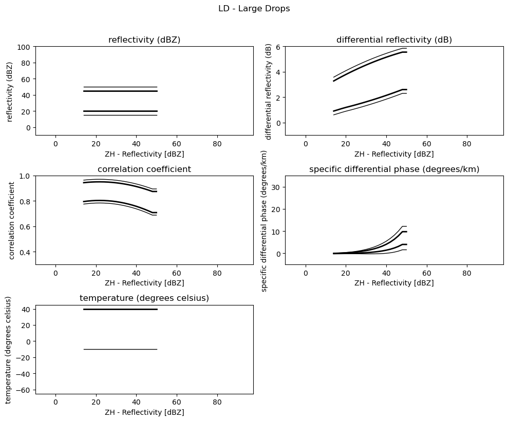
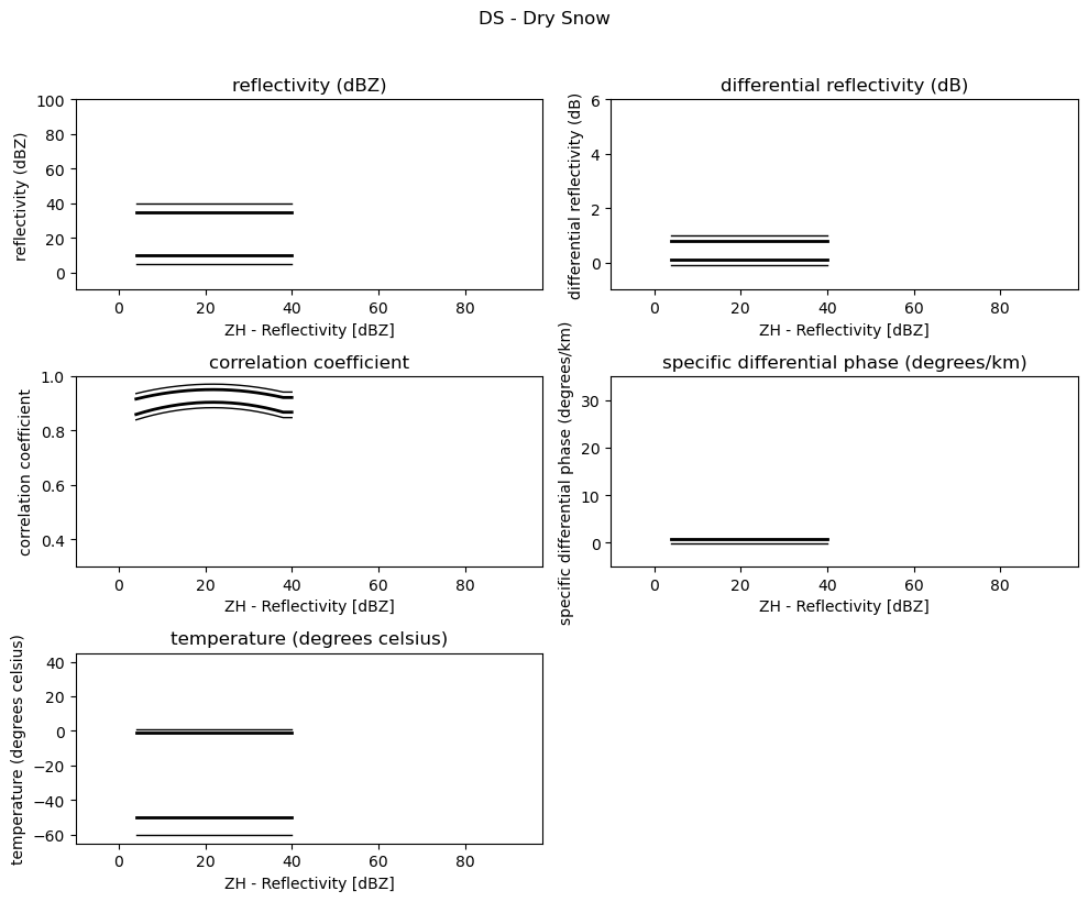
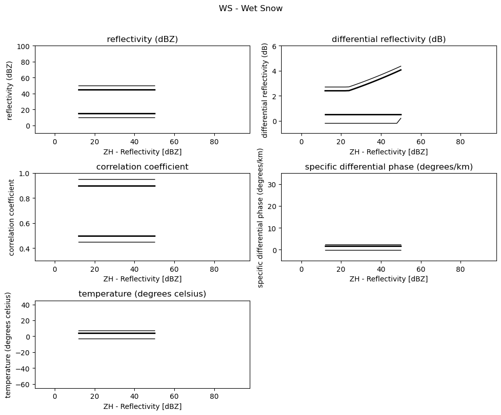
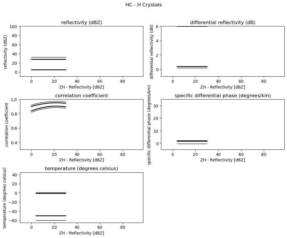
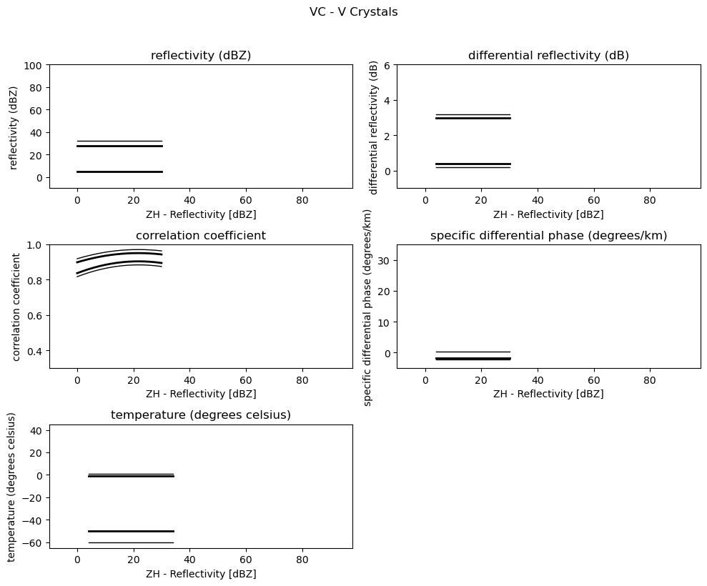
The hydrometeorclassification code is based on the paper by Zrnic et.al 2001 utilizing 2D trapezoidal membership functions based on the paper by Straka et. al 2000 adapted by Evaristo et. al 2013 for X-Band.
Precipitation Types
[2]:
pr_types = wrl.classify.pr_types
for k, v in pr_types.items():
    print(str(k) + " - ".join(v))
0LR - Light Rain
1MR - Moderate Rain
2HR - Heavy Rain
3LD - Large Drops
4HL - Hail
5RH - Rain/Hail
6GH - Graupel/Hail
7DS - Dry Snow
8WS - Wet Snow
9HC - H Crystals
10VC - V Crystals
11NP - No Precip
Membership Functions
Load 2D Membership Functions
[3]:
filename = wrl.util.get_wradlib_data_file("misc/msf_xband.gz")
msf = wrl.io.get_membership_functions(filename)
Downloading file 'misc/msf_xband.gz' from 'https://github.com/wradlib/wradlib-data/raw/pooch/data/misc/msf_xband.gz' to '/home/runner/work/wradlib-notebooks/wradlib-notebooks/wradlib-data'.
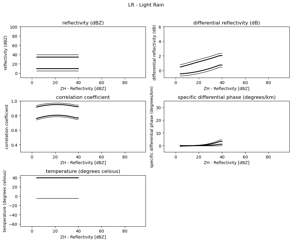
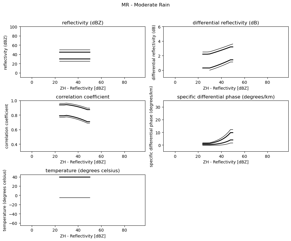
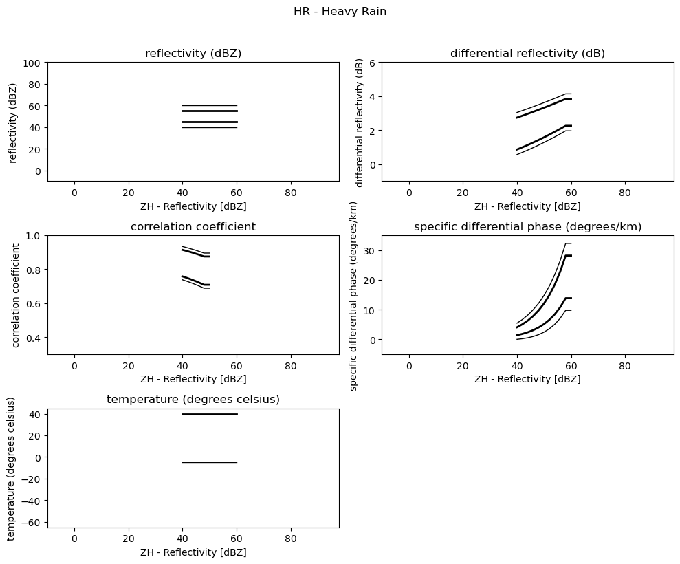
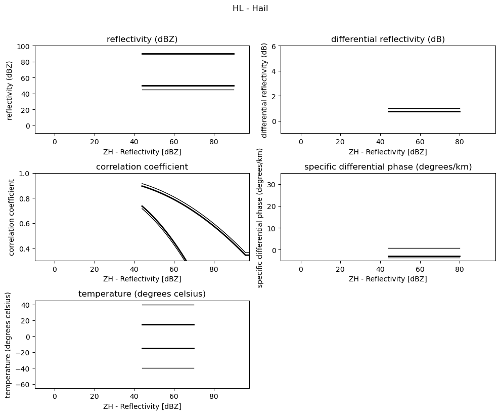
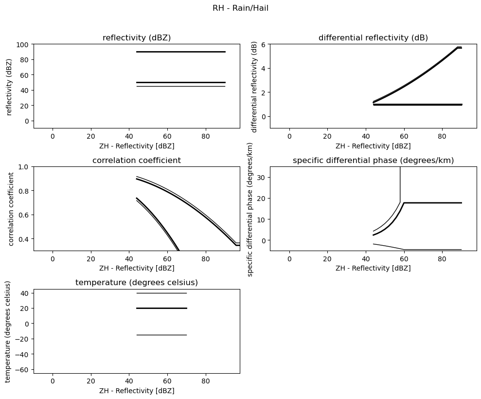
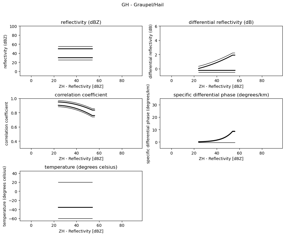
Plot 2D Membership Functions
[4]:
obs = [
    "reflectivity (dBZ)",
    "differential reflectivity (dB)",
    "correlation coefficient",
    "specific differential phase (degrees/km)",
    "temperature (degrees celsius)",
]
minmax = [(-10, 100), (-1, 6), (0.3, 1.0), (-5, 35), (-65, 45)]

for i, v in enumerate(msf):
    fig = pl.figure(figsize=(10, 8))
    t = fig.suptitle(" - ".join(pr_types[i]))
    t.set_y(1.02)
    for k, p in enumerate(v):
        ax = fig.add_subplot(3, 2, k + 1)
        ax.plot(p[:, 0], np.ma.masked_equal(p[:, 1], 0.0), "k", lw=1.0)
        ax.plot(p[:, 0], np.ma.masked_equal(p[:, 2], 0.0), "k", lw=2.0)
        ax.plot(p[:, 0], np.ma.masked_equal(p[:, 3], 0.0), "k", lw=2.0)
        ax.plot(p[:, 0], np.ma.masked_equal(p[:, 4], 0.0), "k", lw=1.0)

        ax.set_xlim((p[:, 0].min(), p[:, 0].max()))
        ax.margins(x=0.05, y=0.05)
        ax.set_xlabel("ZH - Reflectivity [dBZ]")
        ax.set_ylabel(obs[k])
        t = ax.set_title(obs[k])
        ax.set_ylim(minmax[k])
    fig.tight_layout()
pl.show()
Use Sounding Data
Retrieve Sounding Data
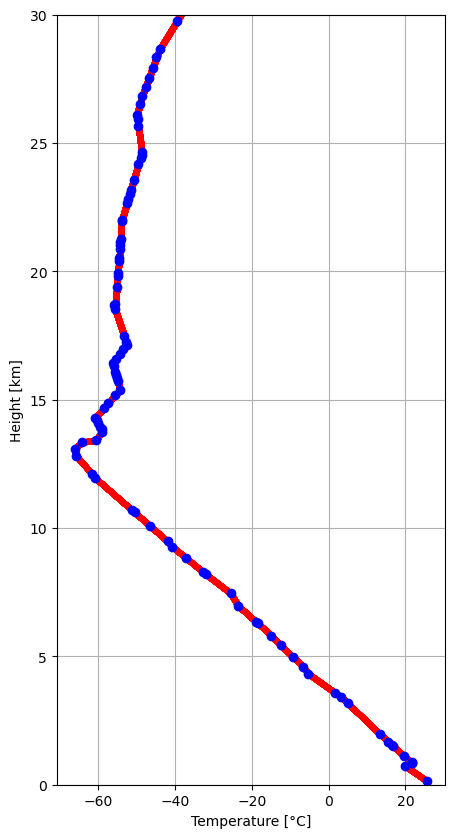
To get the temperature as additional discriminator we use radiosonde data from the University of Wyoming.
The function get_radiosonde tries to find the next next available radiosonde measurement on the given date.
[5]:
rs_time = dt.datetime(2014, 6, 10, 12, 0)
import urllib

try:
    rs_data, rs_meta = wrl.io.get_radiosonde(10410, rs_time)
except urllib.error.HTTPError:
    dataf = wrl.util.get_wradlib_data_file("misc/radiosonde_10410_20140610_1200.h5")
    rs_data, _ = wrl.io.from_hdf5(dataf)
    metaf = wrl.util.get_wradlib_data_file("misc/radiosonde_10410_20140610_1200.json")
    with open(metaf, "r") as infile:
        import json

        rs_meta = json.load(infile)
rs_meta
[5]:
{'Station identifier': 'EDZE',
 'Station number': 10410,
 'Observation time': datetime.datetime(2014, 6, 10, 12, 0),
 'Station latitude': 51.4,
 'Station longitude': 6.97,
 'Station elevation': 147.0,
 'Showalter index': 1.65,
 'Lifted index': -5.85,
 'LIFT computed using virtual temperature': -6.24,
 'SWEAT index': 89.02,
 'K index': 23.7,
 'Cross totals index': 17.3,
 'Vertical totals index': 31.3,
 'Totals totals index': 48.6,
 'Convective Available Potential Energy': 1542.9,
 'CAPE using virtual temperature': 1644.44,
 'Convective Inhibition': -139.39,
 'CINS using virtual temperature': -79.9,
 'Equilibrum Level': 202.46,
 'Equilibrum Level using virtual temperature': 202.39,
 'Level of Free Convection': 736.36,
 'LFCT using virtual temperature': 773.09,
 'Bulk Richardson Number': 57.4,
 'Bulk Richardson Number using CAPV': 61.18,
 'Temp [K] of the Lifted Condensation Level': 288.22,
 'Pres [hPa] of the Lifted Condensation Level': 882.28,
 'Equivalent potential temp [K] of the LCL': 334.9,
 'Mean mixed layer potential temperature': 298.74,
 'Mean mixed layer mixing ratio': 12.42,
 '1000 hPa to 500 hPa thickness': 5663.0,
 'Precipitable water [mm] for entire sounding': 28.11,
 'quantity': {'PRES': 'hPa',
  'HGHT': 'm',
  'TEMP': 'C',
  'DWPT': 'C',
  'FRPT': 'C',
  'RELH': '%',
  'RELI': '%',
  'MIXR': 'g/kg',
  'DRCT': 'deg',
  'SKNT': 'knot',
  'THTA': 'K',
  'THTE': 'K',
  'THTV': 'K'}}
Extract Temperature and Height
[6]:
stemp = rs_data["TEMP"]
sheight = rs_data["HGHT"]
# remove nans
idx = np.isfinite(stemp)
stemp = stemp[idx]
sheight = sheight[idx]
Interpolate to higher resolution
[7]:
# highres height
hmax = 30000.0
ht = np.arange(0.0, hmax)

ipolfunc = interpolate.interp1d(sheight, stemp, kind="linear", bounds_error=False)
itemp = ipolfunc(ht)
Fix Temperature below first measurement
[8]:
first = np.nanargmax(itemp)
itemp[0:first] = itemp[first]
Plot Temperature Profile
[9]:
fig = pl.figure(figsize=(5, 10))
ax = fig.add_subplot(111)
l1 = ax.plot(itemp, ht / 1000, "r.")
l2 = ax.plot(stemp, sheight / 1000, "bo")
ax.set_xlabel("Temperature [°C]")
ax.set_ylabel("Height [km]")
ax.set_ylim(0, hmax / 1000)
ax.grid()
pl.show()
Prepare Radar Data
Load Radar Data
[10]:
# read the radar volume scan
filename = "hdf5/2014-06-09--185000.rhi.mvol"
filename = wrl.util.get_wradlib_data_file(filename)
Downloading file 'hdf5/2014-06-09--185000.rhi.mvol' from 'https://github.com/wradlib/wradlib-data/raw/pooch/data/hdf5/2014-06-09--185000.rhi.mvol' to '/home/runner/work/wradlib-notebooks/wradlib-notebooks/wradlib-data'.
Extract data for georeferencing
[11]:
data, meta = wrl.io.read_gamic_hdf5(filename)
r = meta["SCAN0"]["r"] - meta["SCAN0"]["bin_range"] / 2.0
el = meta["SCAN0"]["el"]
az = meta["SCAN0"]["az"]
rays = meta["SCAN0"]["ray_count"]
bins = meta["SCAN0"]["bin_count"]
sitecoords = (meta["VOL"]["Longitude"], meta["VOL"]["Latitude"], meta["VOL"]["Height"])
Get Heights of Radar Bins
[12]:
re = wrl.georef.get_earth_radius(sitecoords[1])
print(r.shape, el.shape)
bheight = wrl.georef.bin_altitude(r[:, np.newaxis], el, sitecoords[2], re).T
print(bheight.shape)
(667,) (450,)
(450, 667)
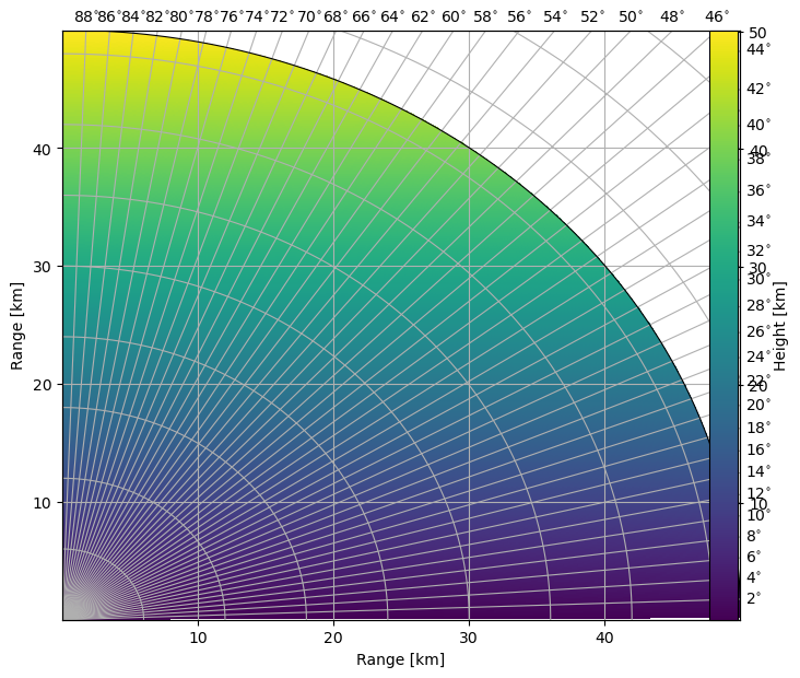
Plot RHI of Heights
[13]:
fig = pl.figure(figsize=(8, 7))
cmap = mpl.cm.viridis
cgax, im = wrl.vis.plot_rhi(
    bheight / 1000.0, r=r / 1000.0, th=el, proj="cg", cmap=cmap, ax=111, fig=fig
)
cbar = pl.colorbar(im, fraction=0.046, pad=0.1)
cbar.set_label("Height [km]")
caax = cgax.parasites[0]
caax.set_xlabel("Range [km]")
caax.set_ylabel("Range [km]")
pl.show()
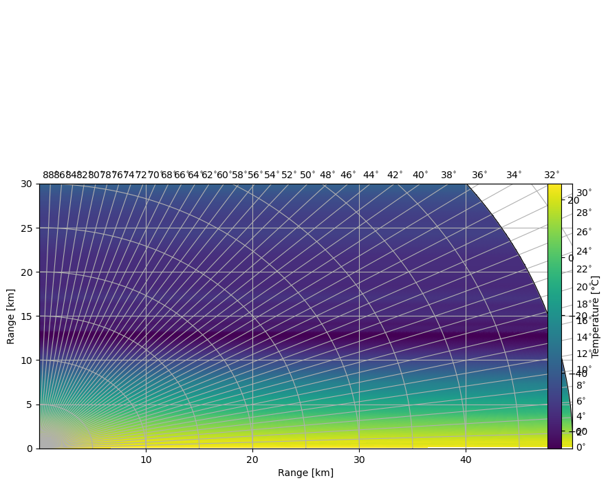
Get Index into High Res Height Array
[14]:
idx = np.digitize(bheight, ht)
print(idx.shape, ht.shape, itemp.shape)
rtemp = itemp[idx - 1]
print(rtemp.min())
(450, 667) (30000,) (30000,)
-66.1
Plot RHI of Temperatures
[15]:
fig = pl.figure(figsize=(10, 5))
cgax, im = wrl.vis.plot_rhi(
    rtemp, r=r / 1000.0, th=el, proj="cg", cmap=cmap, ax=111, fig=fig
)
cbar = pl.colorbar(im, fraction=0.046, pad=0.1)
cbar.set_label("Temperature [°C]")
caax = cgax.parasites[0]
caax.set_xlabel("Range [km]")
caax.set_ylabel("Range [km]")
cgax.set_ylim(0, hmax / 1000)
pl.show()
HMC Workflow
Stack Observables
[16]:
hmca = np.vstack(
    (
        data["SCAN0"]["ZH"]["data"][np.newaxis, ...],
        data["SCAN0"]["ZDR"]["data"][np.newaxis, ...],
        data["SCAN0"]["RHOHV"]["data"][np.newaxis, ...],
        data["SCAN0"]["KDP"]["data"][np.newaxis, ...],
        rtemp[np.newaxis, ...],
    )
)
print(hmca.shape)
(5, 450, 667)
Setup Independent Observable \(Z_H\)
[17]:
msf_idp = msf[0, 0, :, 0]
msf_obs = msf[..., 1:]
Retrieve membership function values based on independent observable
[18]:
msf_val = wrl.classify.msf_index_indep(msf_obs, msf_idp, hmca[0])
Fuzzyfication
[19]:
fu = wrl.classify.fuzzyfi(msf_val, hmca)
Probability
[20]:
# Weights
w = np.array([2.0, 1.0, 1.0, 1.0, 1.0])
prob = wrl.classify.probability(fu, w)
Classification
[21]:
hmc_idx, hmc_vals = wrl.classify.classify(prob, threshold=0.0)
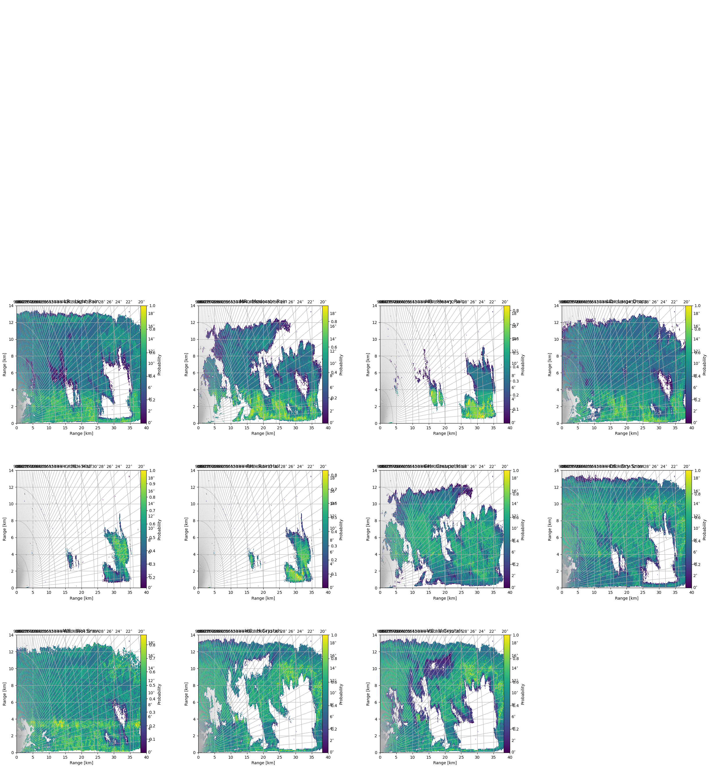
Plot HMC Results
Plot Probability of HMC Types
[22]:
fig = pl.figure(figsize=(30, 20))
import matplotlib.gridspec as gridspec

gs = gridspec.GridSpec(3, 4, wspace=0.4, hspace=0.4)
for i, c in enumerate(prob):
    cgax, im = wrl.vis.plot_rhi(
        np.ma.masked_less_equal(c, 0.0),
        r=r / 1000.0,
        th=el,
        proj="cg",
        ax=gs[i],
        fig=fig,
    )
    cbar = pl.colorbar(im, fraction=0.046, pad=0.15)
    cbar.set_label("Probability")
    caax = cgax.parasites[0]
    caax.set_xlabel("Range [km]")
    caax.set_ylabel("Range [km]")
    t = cgax.set_title(" - ".join(pr_types[i]))
    t.set_y(1.1)
    cgax.set_xlim(0, 40)
    cgax.set_ylim(0, 14)
pl.show()
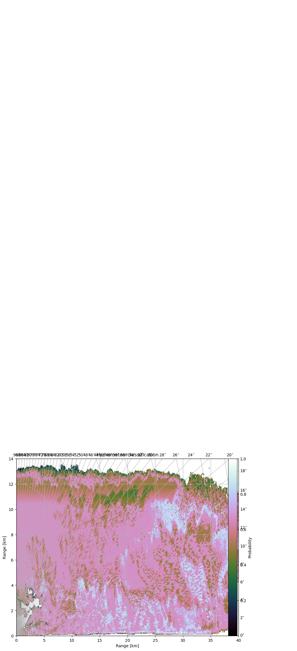
Plot maximum probability
[23]:
fig = pl.figure(figsize=(10, 8))
cgax, im = wrl.vis.plot_rhi(
    hmc_vals[11], ax=111, proj="cg", r=r / 1000.0, th=el, cmap="cubehelix", fig=fig
)
cbar = pl.colorbar(im, fraction=0.046, pad=0.1)
cbar.set_label("Probability")
caax = cgax.parasites[0]
caax.set_xlabel("Range [km]")
caax.set_ylabel("Range [km]")
t = cgax.set_title("Hydrometeorclassification")
t.set_y(1.05)
cgax.set_xlim(0, 40)
cgax.set_ylim(0, 14)
pl.show()
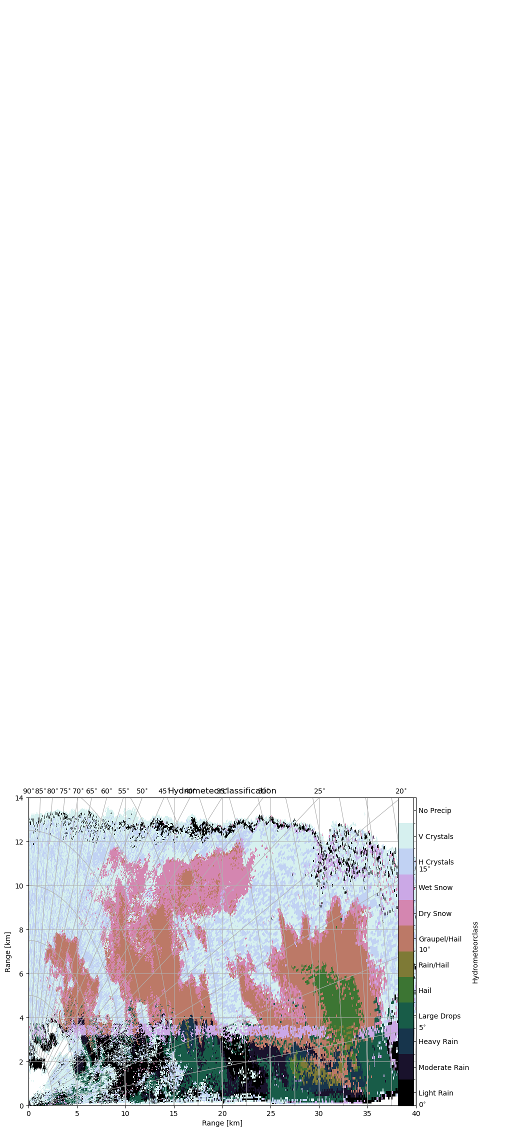
Plot classification result
[24]:
bounds = np.arange(-0.5, prob.shape[0] + 0.6, 1)
ticks = np.arange(0, prob.shape[0] + 1)
cmap = mpl.cm.get_cmap("cubehelix", len(ticks))
norm = mpl.colors.BoundaryNorm(bounds, cmap.N)
[25]:
fig = pl.figure(figsize=(10, 8))
cgax, im = wrl.vis.plot_rhi(
    hmc_idx[11],
    ax=111,
    proj={"angular_spacing": 20.0, "radial_spacing": 12.0, "latmin": 2.5},
    r=r / 1000.0,
    th=el,
    norm=norm,
    cmap=cmap,
    fig=fig,
)
cbar = pl.colorbar(im, ticks=ticks, fraction=0.046, norm=norm, pad=0.1)
cbar.set_label("Hydrometeorclass")
caax = cgax.parasites[0]
caax.set_xlabel("Range [km]")
caax.set_ylabel("Range [km]")
labels = [pr_types[i][1] for i, _ in enumerate(pr_types)]
labels = cbar.ax.set_yticklabels(labels)
t = cgax.set_title("Hydrometeorclassification")
t.set_y(1.05)
cgax.set_xlim(0, 40)
cgax.set_ylim(0, 14)
pl.show()