Beam Blockage Calculation using a DEM

Here, we derive (partial) beam-blockage (PBB) from a Digital Elevation Model (DEM).

We require - the local radar setup (sitecoords, number of rays, number of bins, antenna elevation, beamwidth, and the range resolution); - a DEM with a adequate resolution.

Here we use pre-processed data from the GTOPO30 and SRTM missions.

import wradlib as wrl
import matplotlib.pyplot as pl
import matplotlib as mpl
import warnings

warnings.filterwarnings("ignore")
try:
    get_ipython().run_line_magic("matplotlib inline")
except:
    pl.ion()
import numpy as np

/home/runner/micromamba-root/envs/wradlib-notebooks/lib/python3.11/site-packages/tqdm/auto.py:22: TqdmWarning: IProgress not found. Please update jupyter and ipywidgets. See https://ipywidgets.readthedocs.io/en/stable/user_install.html
  from .autonotebook import tqdm as notebook_tqdm

Setup for Bonn radar

First, we need to define some radar specifications (here: University of Bonn).

sitecoords = (7.071663, 50.73052, 99.5)
nrays = 360  # number of rays
nbins = 1000  # number of range bins
el = 1.0  # vertical antenna pointing angle (deg)
bw = 1.0  # half power beam width (deg)
range_res = 100.0  # range resolution (meters)

Create the range, azimuth, and beamradius arrays.

r = np.arange(nbins) * range_res
beamradius = wrl.util.half_power_radius(r, bw)

We use

• wradlib.georef.sweep_centroids and

• wradlib.georef.spherical_to_proj

to calculate the spherical coordinates of the bin centroids and their longitude, latitude and altitude.

coord = wrl.georef.sweep_centroids(nrays, range_res, nbins, el)
coords = wrl.georef.spherical_to_proj(
    coord[..., 0], coord[..., 1], coord[..., 2], sitecoords
)
lon = coords[..., 0]
lat = coords[..., 1]
alt = coords[..., 2]

polcoords = coords[..., :2]
print("lon,lat,alt:", coords.shape)

lon,lat,alt: (360, 1000, 3)

rlimits = (lon.min(), lat.min(), lon.max(), lat.max())
print(
    "Radar bounding box:\n\t%.2f\n%.2f             %.2f\n\t%.2f"
    % (lat.max(), lon.min(), lon.max(), lat.min())
)

Radar bounding box:
        51.63
5.66             8.49
        49.83

Preprocessing the digitial elevation model

• Read the DEM from a geotiff file (in WRADLIB_DATA);

• clip the region inside the bounding box;

• map the DEM values to the polar grid points.

Note: You can choose between the coarser resolution bonn_gtopo.tif (from GTOPO30) and the finer resolution bonn_new.tif (from the SRTM mission).

The DEM raster data is opened via wradlib.io.open_raster and extracted via wradlib.georef.extract_raster_dataset.

# rasterfile = wrl.util.get_wradlib_data_file('geo/bonn_gtopo.tif')
rasterfile = wrl.util.get_wradlib_data_file("geo/bonn_new.tif")

ds = wrl.io.open_raster(rasterfile)
rastervalues, rastercoords, proj = wrl.georef.extract_raster_dataset(
    ds, nodata=-32768.0
)

# Clip the region inside our bounding box
ind = wrl.util.find_bbox_indices(rastercoords, rlimits)
rastercoords = rastercoords[ind[1] : ind[3], ind[0] : ind[2], ...]
rastervalues = rastervalues[ind[1] : ind[3], ind[0] : ind[2]]

# Map rastervalues to polar grid points
polarvalues = wrl.ipol.cart_to_irregular_spline(
    rastercoords, rastervalues, polcoords, order=3, prefilter=False
)

Downloading file 'geo/bonn_new.tif' from 'https://github.com/wradlib/wradlib-data/raw/pooch/data/geo/bonn_new.tif' to '/home/runner/work/wradlib-notebooks/wradlib-notebooks/wradlib-data'.

Calculate Beam-Blockage

Now we can finally apply the wradlib.qual.beam_block_frac function to calculate the PBB.

PBB = wrl.qual.beam_block_frac(polarvalues, alt, beamradius)
PBB = np.ma.masked_invalid(PBB)
print(PBB.shape)

(360, 1000)

So far, we calculated the fraction of beam blockage for each bin.

But we need to into account that the radar signal travels along a beam. Cumulative beam blockage (CBB) in one bin along a beam will always be at least as high as the maximum PBB of the preceeding bins (see wradlib.qual.cum_beam_block_frac)

CBB = wrl.qual.cum_beam_block_frac(PBB)
print(CBB.shape)

(360, 1000)

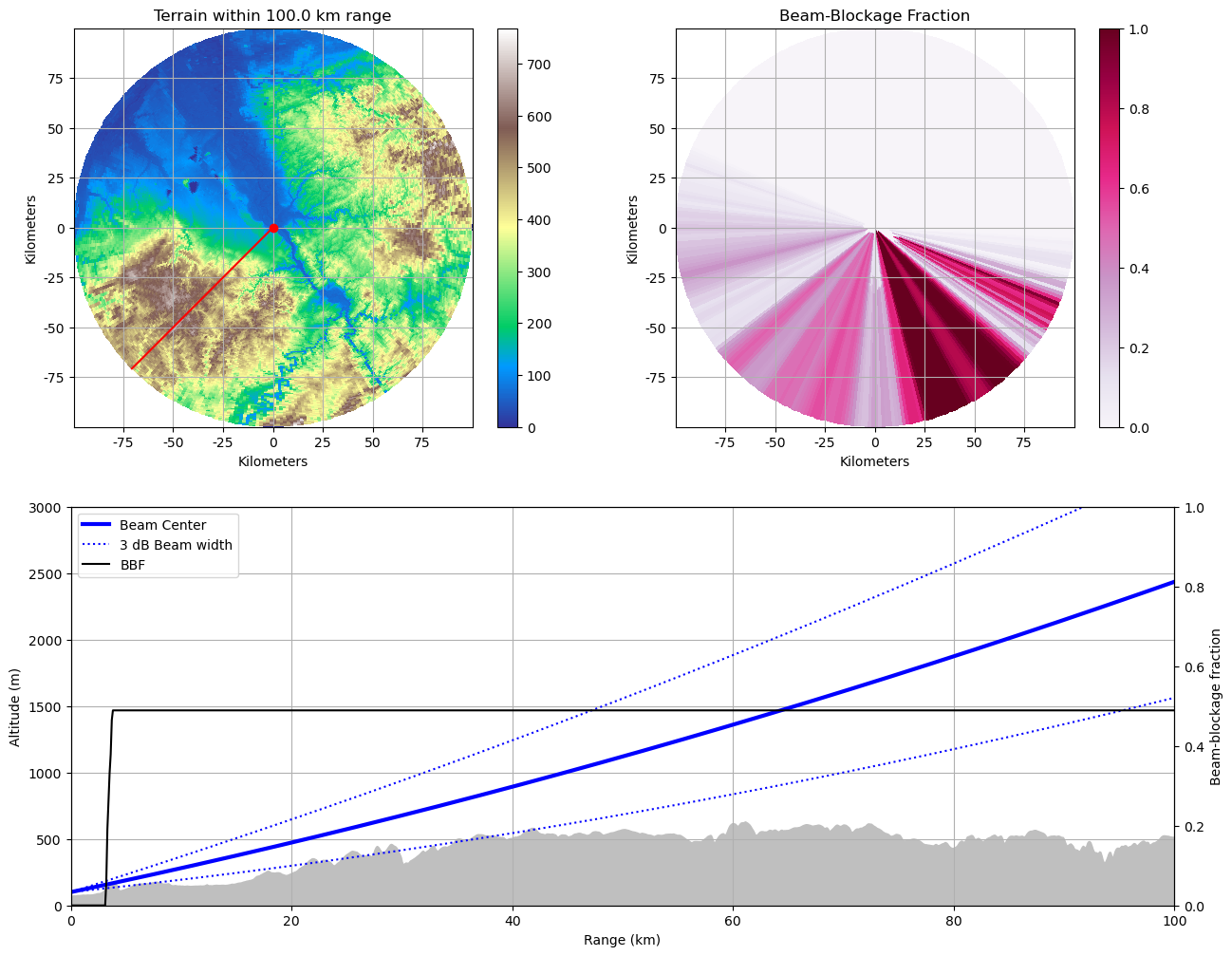
Visualize Beamblockage

Now we visualize - the average terrain altitude per radar bin - a beam blockage map - interaction with terrain along a single beam

# just a little helper function to style x and y axes of our maps
def annotate_map(ax, cm=None, title=""):
    ticks = (ax.get_xticks() / 1000).astype(int)
    ax.set_xticklabels(ticks)
    ticks = (ax.get_yticks() / 1000).astype(int)
    ax.set_yticklabels(ticks)
    ax.set_xlabel("Kilometers")
    ax.set_ylabel("Kilometers")
    if not cm is None:
        pl.colorbar(cm, ax=ax)
    if not title == "":
        ax.set_title(title)
    ax.grid()

fig = pl.figure(figsize=(15, 12))

# create subplots
ax1 = pl.subplot2grid((2, 2), (0, 0))
ax2 = pl.subplot2grid((2, 2), (0, 1))
ax3 = pl.subplot2grid((2, 2), (1, 0), colspan=2, rowspan=1)

# azimuth angle
angle = 225

# Plot terrain (on ax1)
ax1, dem = wrl.vis.plot_ppi(
    polarvalues, ax=ax1, r=r, az=coord[:, 0, 1], cmap=mpl.cm.terrain, vmin=0.0
)
ax1.plot(
    [0, np.sin(np.radians(angle)) * 1e5], [0, np.cos(np.radians(angle)) * 1e5], "r-"
)
ax1.plot(sitecoords[0], sitecoords[1], "ro")
annotate_map(ax1, dem, "Terrain within {0} km range".format(np.max(r / 1000.0) + 0.1))

# Plot CBB (on ax2)
ax2, cbb = wrl.vis.plot_ppi(
    CBB, ax=ax2, r=r, az=coord[:, 0, 1], cmap=mpl.cm.PuRd, vmin=0, vmax=1
)
annotate_map(ax2, cbb, "Beam-Blockage Fraction")

# Plot single ray terrain profile on ax3
(bc,) = ax3.plot(r / 1000.0, alt[angle, :], "-b", linewidth=3, label="Beam Center")
(b3db,) = ax3.plot(
    r / 1000.0,
    (alt[angle, :] + beamradius),
    ":b",
    linewidth=1.5,
    label="3 dB Beam width",
)
ax3.plot(r / 1000.0, (alt[angle, :] - beamradius), ":b")
ax3.fill_between(r / 1000.0, 0.0, polarvalues[angle, :], color="0.75")
ax3.set_xlim(0.0, np.max(r / 1000.0) + 0.1)
ax3.set_ylim(0.0, 3000)
ax3.set_xlabel("Range (km)")
ax3.set_ylabel("Altitude (m)")
ax3.grid()

axb = ax3.twinx()
(bbf,) = axb.plot(r / 1000.0, CBB[angle, :], "-k", label="BBF")
axb.set_ylabel("Beam-blockage fraction")
axb.set_ylim(0.0, 1.0)
axb.set_xlim(0.0, np.max(r / 1000.0) + 0.1)


legend = ax3.legend(
    (bc, b3db, bbf),
    ("Beam Center", "3 dB Beam width", "BBF"),
    loc="upper left",
    fontsize=10,
)

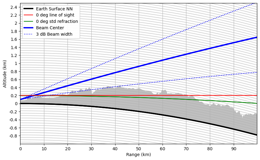
Visualize Beam Propagation showing earth curvature

Now we visualize - interaction with terrain along a single beam

In this representation the earth curvature is shown. For this we assume the earth a sphere with exactly 6370000 m radius. This is needed to get the height ticks at nice position.

def height_formatter(x, pos):
    x = (x - 6370000) / 1000
    fmt_str = "{:g}".format(x)
    return fmt_str


def range_formatter(x, pos):
    x = x / 1000.0
    fmt_str = "{:g}".format(x)
    return fmt_str

• The wradlib.vis.create_cg-function is facilitated to create the curved geometries.

• The actual data is plottet as (theta, range) on the parasite axis.

• Some tweaking is needed to get the final plot look nice.

fig = pl.figure(figsize=(10, 6))

cgax, caax, paax = wrl.vis.create_cg(fig=fig, rot=0, scale=1)

# azimuth angle
angle = 225

# fix grid_helper
er = 6370000
gh = cgax.get_grid_helper()
gh.grid_finder.grid_locator2._nbins = 80
gh.grid_finder.grid_locator2._steps = [1, 2, 4, 5, 10]

# calculate beam_height and arc_distance for ke=1
# means line of sight
bhe = wrl.georef.bin_altitude(r, 0, sitecoords[2], re=er, ke=1.0)
ade = wrl.georef.bin_distance(r, 0, sitecoords[2], re=er, ke=1.0)
nn0 = np.zeros_like(r)
# for nice plotting we assume earth_radius = 6370000 m
ecp = nn0 + er
# theta (arc_distance sector angle)
thetap = -np.degrees(ade / er) + 90.0

# zero degree elevation with standard refraction
bh0 = wrl.georef.bin_altitude(r, 0, sitecoords[2], re=er)

# plot (ecp is earth surface normal null)
(bes,) = paax.plot(thetap, ecp, "-k", linewidth=3, label="Earth Surface NN")
(bc,) = paax.plot(thetap, ecp + alt[angle, :], "-b", linewidth=3, label="Beam Center")
(bc0r,) = paax.plot(thetap, ecp + bh0 + alt[angle, 0], "-g", label="0 deg Refraction")
(bc0n,) = paax.plot(
    thetap, ecp + bhe + alt[angle, 0], "-r", label="0 deg line of sight"
)
(b3db,) = paax.plot(
    thetap, ecp + alt[angle, :] + beamradius, ":b", label="+3 dB Beam width"
)
paax.plot(thetap, ecp + alt[angle, :] - beamradius, ":b", label="-3 dB Beam width")

# orography
paax.fill_between(thetap, ecp, ecp + polarvalues[angle, :], color="0.75")

# shape axes
cgax.set_xlim(0, np.max(ade))
cgax.set_ylim([ecp.min() - 1000, ecp.max() + 2500])
caax.grid(True, axis="x")
cgax.grid(True, axis="y")
cgax.axis["top"].toggle(all=False)
caax.yaxis.set_major_locator(
    mpl.ticker.MaxNLocator(steps=[1, 2, 4, 5, 10], nbins=20, prune="both")
)
caax.xaxis.set_major_locator(mpl.ticker.MaxNLocator())
caax.yaxis.set_major_formatter(mpl.ticker.FuncFormatter(height_formatter))
caax.xaxis.set_major_formatter(mpl.ticker.FuncFormatter(range_formatter))

caax.set_xlabel("Range (km)")
caax.set_ylabel("Altitude (km)")

legend = paax.legend(
    (bes, bc0n, bc0r, bc, b3db),
    (
        "Earth Surface NN",
        "0 deg line of sight",
        "0 deg std refraction",
        "Beam Center",
        "3 dB Beam width",
    ),
    loc="upper left",
    fontsize=10,
)

Go back to Read DEM Raster Data, change the rasterfile to use the other resolution DEM and process again.